

156
5 Vibration of Two Degrees of Freedom System
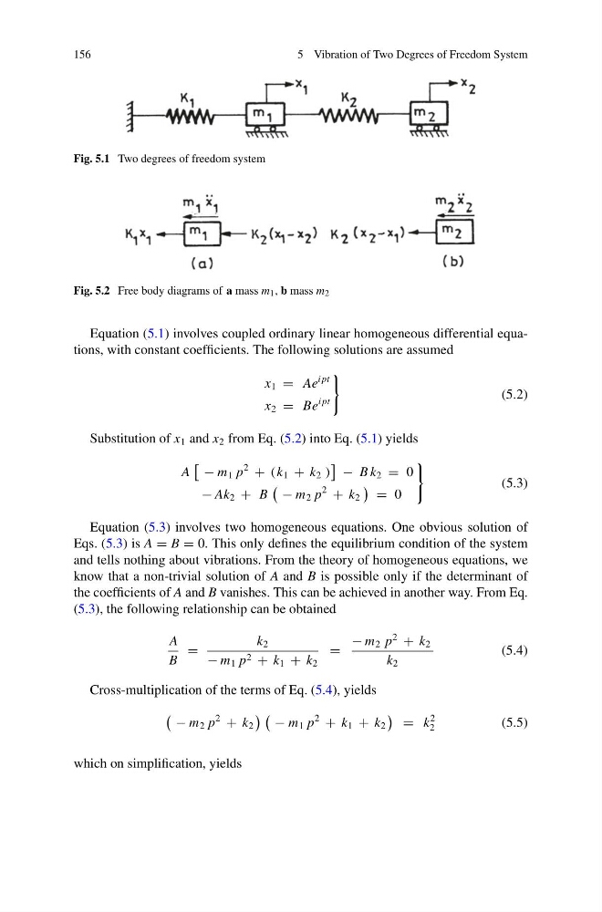
Fig. 5.1 Two degrees of freedom system
Fig. 5.2 Free body diagrams of a mass m 1 , b mass m 2
Equation (5.1) involves coupled ordinary linear homogeneous differential equations, with constant coefficients. The following solutions are assumed
x 1 = Ae
i pt
x 2 = Be
i pt
(5.2)
Substitution of x 1 and x 2 from Eq. (5.2) into Eq. (5.1) yields
A
− m 1 p
2
+ ( k 1 + k 2 )
− B k 2 = 0
− Ak 2 + B
− m 2 p
2
+ k 2
= 0
(5.3)
Equation (5.3) involves two homogeneous equations. One obvious solution of
Eqs. (5.3) is A = B = 0. This only defines the equilibrium condition of the system
and tells nothing about vibrations. From the theory of homogeneous equations, we
know that a non-trivial solution of A and B is possible only if the determinant of
the coefficients of A and B vanishes. This can be achieved in another way. From Eq.
(5.3), the following relationship can be obtained
A
B
=
k 2
− m 1 p 2 + k 1 + k 2
=
− m 2 p
2
+ k 2
k 2
(5.4)
Cross-multiplication of the terms of Eq. (5.4), yields
− m 2 p
2
+ k 2
− m 1 p
2
+ k 1 + k 2
= k
2
2
(5.5)
which on simplification, yields
5 Vibration of Two Degrees of Freedom System
Fig. 5.1 Two degrees of freedom system
Fig. 5.2 Free body diagrams of a mass m 1 , b mass m 2
Equation (5.1) involves coupled ordinary linear homogeneous differential equations, with constant coefficients. The following solutions are assumed
x 1 = Ae
i pt
x 2 = Be
i pt
(5.2)
Substitution of x 1 and x 2 from Eq. (5.2) into Eq. (5.1) yields
A
− m 1 p
2
+ ( k 1 + k 2 )
− B k 2 = 0
− Ak 2 + B
− m 2 p
2
+ k 2
= 0
(5.3)
Equation (5.3) involves two homogeneous equations. One obvious solution of
Eqs. (5.3) is A = B = 0. This only defines the equilibrium condition of the system
and tells nothing about vibrations. From the theory of homogeneous equations, we
know that a non-trivial solution of A and B is possible only if the determinant of
the coefficients of A and B vanishes. This can be achieved in another way. From Eq.
(5.3), the following relationship can be obtained
A
B
=
k 2
− m 1 p 2 + k 1 + k 2
=
− m 2 p
2
+ k 2
k 2
(5.4)
Cross-multiplication of the terms of Eq. (5.4), yields
− m 2 p
2
+ k 2
− m 1 p
2
+ k 1 + k 2
= k
2
2
(5.5)
which on simplification, yields