

4.2 Direct Integration Techniques
135
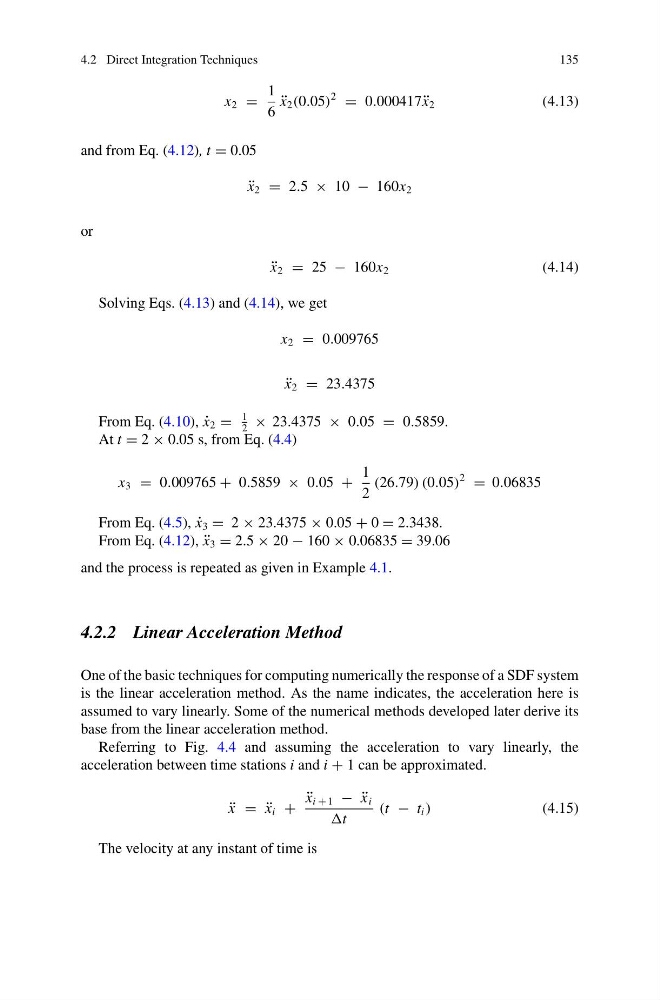
x 2 =
1
6
¨
x 2 (0.05)
2
= 0.000417 ¨
x 2
(4.13)
and from Eq. (4.12), t = 0.05
¨
x 2 = 2.5 × 10 − 160x 2
or
¨
x 2 = 25 − 160x 2
(4.14)
Solving Eqs. (4.13) and (4.14), we get
x 2 = 0.009765
¨
x 2 = 23.4375
From Eq. (4.10), ˙
x 2 =
1
2
× 23.4375 × 0.05 = 0.5859.
At t = 2 × 0.05 s, from Eq. (4.4)
x 3 = 0.009765 + 0.5859 × 0.05 +
1
2
(26.79) (0.05)
2
= 0.06835
From Eq. (4.5), ˙
x 3 = 2 × 23.4375 × 0.05 + 0 = 2.3438.
From Eq. (4.12), ¨
x 3 = 2.5 × 20 − 160 × 0.06835 = 39.06
and the process is repeated as given in Example 4.1.
4.2.2 Linear Acceleration Method
One of the basic techniques for computing numerically the response of a SDF system
is the linear acceleration method. As the name indicates, the acceleration here is
assumed to vary linearly. Some of the numerical methods developed later derive its
base from the linear acceleration method.
Referring to Fig. 4.4 and assuming the acceleration to vary linearly, the
acceleration between time stations i and i + 1 can be approximated.
¨
x = ¨
x i +
¨
x i + 1 − ¨
x i
t
(t − t i )
(4.15)
The velocity at any instant of time is
135
x 2 =
1
6
¨
x 2 (0.05)
2
= 0.000417 ¨
x 2
(4.13)
and from Eq. (4.12), t = 0.05
¨
x 2 = 2.5 × 10 − 160x 2
or
¨
x 2 = 25 − 160x 2
(4.14)
Solving Eqs. (4.13) and (4.14), we get
x 2 = 0.009765
¨
x 2 = 23.4375
From Eq. (4.10), ˙
x 2 =
1
2
× 23.4375 × 0.05 = 0.5859.
At t = 2 × 0.05 s, from Eq. (4.4)
x 3 = 0.009765 + 0.5859 × 0.05 +
1
2
(26.79) (0.05)
2
= 0.06835
From Eq. (4.5), ˙
x 3 = 2 × 23.4375 × 0.05 + 0 = 2.3438.
From Eq. (4.12), ¨
x 3 = 2.5 × 20 − 160 × 0.06835 = 39.06
and the process is repeated as given in Example 4.1.
4.2.2 Linear Acceleration Method
One of the basic techniques for computing numerically the response of a SDF system
is the linear acceleration method. As the name indicates, the acceleration here is
assumed to vary linearly. Some of the numerical methods developed later derive its
base from the linear acceleration method.
Referring to Fig. 4.4 and assuming the acceleration to vary linearly, the
acceleration between time stations i and i + 1 can be approximated.
¨
x = ¨
x i +
¨
x i + 1 − ¨
x i
t
(t − t i )
(4.15)
The velocity at any instant of time is