

134
4 Numerical Methods in Structural Dynamics …
Table 4.1 Response evaluation by finite difference method
t s
F(t)
X
˙
x
¨
x
0
50
0
0
25
0.02
60
0.005
0.5
25
0.04
70
0.02
1.0
15
0.06
80
0.043
1.1
−3.00
0.08
90
0.0644
0.8
−19.40
0.10
100
0.0765
0.024
−26.52
0.12
87.5
0.0717
−1.037
−27.95
0.14
75
0.0454
−2.155
−7.87
x 4 = 0.02 + 1 × 0.02 +
1
2
× 15(0.02)
2
= 0.043
˙
x 4 = 2 × 15 × 0.02 + 0.5 = 1.1
and the process is repeated and results up to t = 0.14 s is presented in Table 4.1.
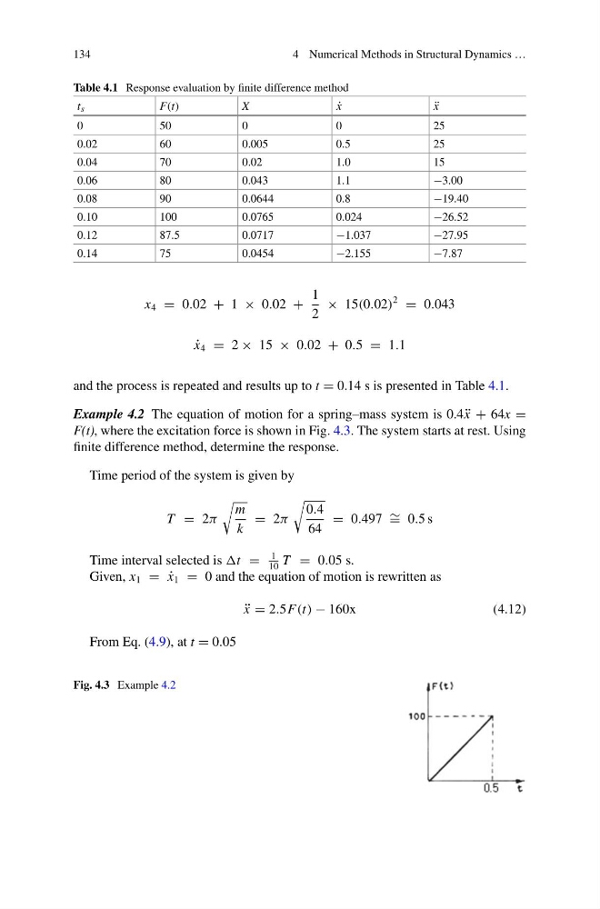
Example 4.2 The equation of motion for a spring–mass system is 0.4 ¨
x + 64x =
F(t), where the excitation force is shown in Fig. 4.3. The system starts at rest. Using
finite difference method, determine the response.
Time period of the system is given by
T = 2π
m
k
= 2π
0.4
64
= 0.497 ∼ = 0.5 s
Time interval selected is t =
1
10
T = 0.05 s.
Given, x 1 = ˙
x 1 = 0 and the equation of motion is rewritten as
¨
x = 2.5F(t) − 160x
(4.12)
From Eq. (4.9), at t = 0.05
Fig. 4.3 Example 4.2
4 Numerical Methods in Structural Dynamics …
Table 4.1 Response evaluation by finite difference method
t s
F(t)
X
˙
x
¨
x
0
50
0
0
25
0.02
60
0.005
0.5
25
0.04
70
0.02
1.0
15
0.06
80
0.043
1.1
−3.00
0.08
90
0.0644
0.8
−19.40
0.10
100
0.0765
0.024
−26.52
0.12
87.5
0.0717
−1.037
−27.95
0.14
75
0.0454
−2.155
−7.87
x 4 = 0.02 + 1 × 0.02 +
1
2
× 15(0.02)
2
= 0.043
˙
x 4 = 2 × 15 × 0.02 + 0.5 = 1.1
and the process is repeated and results up to t = 0.14 s is presented in Table 4.1.
Example 4.2 The equation of motion for a spring–mass system is 0.4 ¨
x + 64x =
F(t), where the excitation force is shown in Fig. 4.3. The system starts at rest. Using
finite difference method, determine the response.
Time period of the system is given by
T = 2π
m
k
= 2π
0.4
64
= 0.497 ∼ = 0.5 s
Time interval selected is t =
1
10
T = 0.05 s.
Given, x 1 = ˙
x 1 = 0 and the equation of motion is rewritten as
¨
x = 2.5F(t) − 160x
(4.12)
From Eq. (4.9), at t = 0.05
Fig. 4.3 Example 4.2