

102
3 Forced Vibration of Single Degree of Freedom System
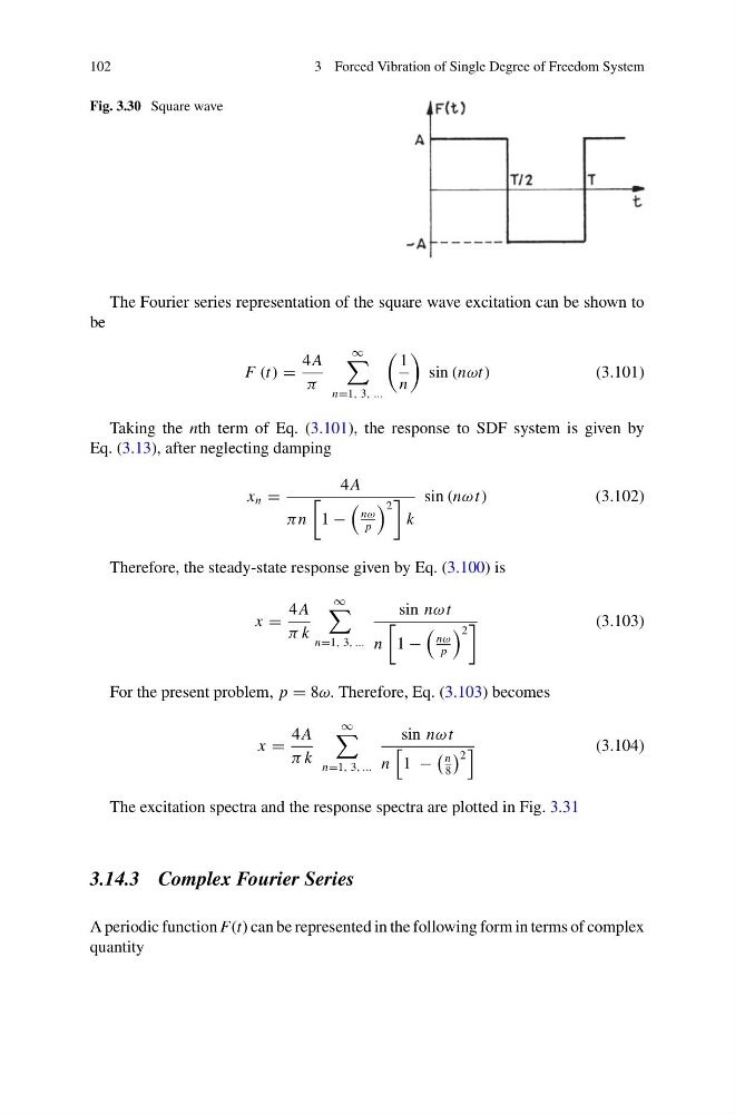
Fig. 3.30 Square wave
The Fourier series representation of the square wave excitation can be shown to
be
F (t) =
4 A
π
∞
n=1, 3, ...
1
n
sin (nωt)
(3.101)
Taking the nth term of Eq. (3.101), the response to SDF system is given by
Eq. (3.13), after neglecting damping
x n =
4 A
π n
1 −
nω
p
2
k
sin (nω t)
(3.102)
Therefore, the steady-state response given by Eq. (3.100) is
x =
4 A
π k
∞
n=1, 3, ...
sin nω t
n
1 −
nω
p
2
(3.103)
For the present problem, p = 8ω. Therefore, Eq. (3.103) becomes
x =
4 A
π k
∞
n=1, 3, ...
sin nω t
n
1 −
n
8
2
(3.104)
The excitation spectra and the response spectra are plotted in Fig. 3.31
3.14.3 Complex Fourier Series
A periodic function F(t) can be represented in the following form in terms of complex
quantity
3 Forced Vibration of Single Degree of Freedom System
Fig. 3.30 Square wave
The Fourier series representation of the square wave excitation can be shown to
be
F (t) =
4 A
π
∞
n=1, 3, ...
1
n
sin (nωt)
(3.101)
Taking the nth term of Eq. (3.101), the response to SDF system is given by
Eq. (3.13), after neglecting damping
x n =
4 A
π n
1 −
nω
p
2
k
sin (nω t)
(3.102)
Therefore, the steady-state response given by Eq. (3.100) is
x =
4 A
π k
∞
n=1, 3, ...
sin nω t
n
1 −
nω
p
2
(3.103)
For the present problem, p = 8ω. Therefore, Eq. (3.103) becomes
x =
4 A
π k
∞
n=1, 3, ...
sin nω t
n
1 −
n
8
2
(3.104)
The excitation spectra and the response spectra are plotted in Fig. 3.31
3.14.3 Complex Fourier Series
A periodic function F(t) can be represented in the following form in terms of complex
quantity