

3.11 Response of Structures Due to Transient Vibration
91
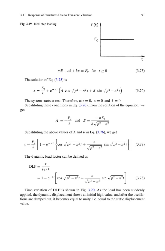
Fig. 3.19 Ideal step loading
m ¨
x + c ˙
x + kx = F 0 for t ≥ 0
(3.75)
The solution of Eq. (3.75) is
x =
F 0
k
+ e
− n t
A cos
p 2 − n 2 t + B sin
p 2 − n 2 t
(3.76)
The system starts at rest. Therefore, at t = 0, x = 0 and ˙
x = 0
Substituting these conditions in Eq. (3.76), from the solution of the equation, we
get
A = −
F 0
k
and B =
− n F 0
k
p 2 − n 2
Substituting the above values of A and B in Eq. (3.76), we get
x =
F 0
k
1 − e
− n t
cos
p 2 − n 2 t +
n
p 2 − n 2
sin
p 2 − n 2 t
(3.77)
The dynamic load factor can be defined as
DLF =
x
F 0 /k
= 1 − e
−n t
cos
p 2 − n 2 t +
n
p 2 − n 2
sin
p 2 − n 2 t
(3.78)
Time variation of DLF is shown in Fig. 3.20. As the load has been suddenly
applied, the dynamic displacement shows an initial high value, and after the oscillations are damped out, it becomes equal to unity, i.e. equal to the static displacement
value.
91
Fig. 3.19 Ideal step loading
m ¨
x + c ˙
x + kx = F 0 for t ≥ 0
(3.75)
The solution of Eq. (3.75) is
x =
F 0
k
+ e
− n t
A cos
p 2 − n 2 t + B sin
p 2 − n 2 t
(3.76)
The system starts at rest. Therefore, at t = 0, x = 0 and ˙
x = 0
Substituting these conditions in Eq. (3.76), from the solution of the equation, we
get
A = −
F 0
k
and B =
− n F 0
k
p 2 − n 2
Substituting the above values of A and B in Eq. (3.76), we get
x =
F 0
k
1 − e
− n t
cos
p 2 − n 2 t +
n
p 2 − n 2
sin
p 2 − n 2 t
(3.77)
The dynamic load factor can be defined as
DLF =
x
F 0 /k
= 1 − e
−n t
cos
p 2 − n 2 t +
n
p 2 − n 2
sin
p 2 − n 2 t
(3.78)
Time variation of DLF is shown in Fig. 3.20. As the load has been suddenly
applied, the dynamic displacement shows an initial high value, and after the oscillations are damped out, it becomes equal to unity, i.e. equal to the static displacement
value.