

must be stressed that although it is not feasible to solve exactly most of the quantum
mechanical problems, methods have been devised to provide approximate solutions
of variable degrees of accuracy, and the entire field of computational chemistry is
built around approximate solutions. Proper modeling requires to know the approximations employed, or at least to be aware of how accurate the results are expected to
be, according to the approximations employed.
The first issue to choose the chemical model is the nature of the system to be
simulated. The most usual way of performing organometallic reactions is employing
molecular species in solution at temperatures often between 0 and 120
C. Simulation
of this kind of reactions is the subject of this chapter. Recent thorough reviews have
addressed the modeling of surface organometallic reactions [28] and heterogenous
catalysis [29]. The larger and the more accurate the model, the more expensive the
calculation. For this reason, the usual way of modeling an organometallic system has
evolved in parallel with the increase of computing power. In the early years of DFT
studies of organometallic reactions, for instance, it was common to model all the
phosphine ligands as PH 3 (“the theoretician phosphine”) to reduce the size of the
system. Nowadays, most of the calculations are performed with the actual molecular
species present in the reaction flask, with no simplification. However, this procedure
is not always enough to assure a proper modeling of the system, as we will show
later on.
Fig. 2 From the flask to the computer: chemical and theoretical models
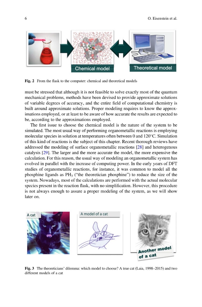
Fig. 3 The theoreticians’ dilemma: which model to choose? A true cat (Laia, 1998–2015) and two
different models of a cat
6
O. Eisenstein et al.
mechanical problems, methods have been devised to provide approximate solutions
of variable degrees of accuracy, and the entire field of computational chemistry is
built around approximate solutions. Proper modeling requires to know the approximations employed, or at least to be aware of how accurate the results are expected to
be, according to the approximations employed.
The first issue to choose the chemical model is the nature of the system to be
simulated. The most usual way of performing organometallic reactions is employing
molecular species in solution at temperatures often between 0 and 120
C. Simulation
of this kind of reactions is the subject of this chapter. Recent thorough reviews have
addressed the modeling of surface organometallic reactions [28] and heterogenous
catalysis [29]. The larger and the more accurate the model, the more expensive the
calculation. For this reason, the usual way of modeling an organometallic system has
evolved in parallel with the increase of computing power. In the early years of DFT
studies of organometallic reactions, for instance, it was common to model all the
phosphine ligands as PH 3 (“the theoretician phosphine”) to reduce the size of the
system. Nowadays, most of the calculations are performed with the actual molecular
species present in the reaction flask, with no simplification. However, this procedure
is not always enough to assure a proper modeling of the system, as we will show
later on.
Fig. 2 From the flask to the computer: chemical and theoretical models
Fig. 3 The theoreticians’ dilemma: which model to choose? A true cat (Laia, 1998–2015) and two
different models of a cat
6
O. Eisenstein et al.