

11 Quantum Mechanics. Algebraic Structure and States
75
More generally, for systems with infinite degrees of freedom and especially for
relativistic quantum systems (where the canonical formalism is problematic, see, e.g.
[S 85]), it is more convenient to identify the algebraic structure, which underlies the
definition of the system, with the algebra (with identity) generated by the physical
quantities, briefly called observables, which can be measured on the given system.
51
From an operational point of view, a system is actually defined by its algebra of
observables A and, by appealing to the operational properties of measurements, one
can argue that A has an identity and can be given the structure of C
∗ -algebra.
52 In
the sequel, we shall take the point of view that a quantum system is defined by its
algebra of observables A, with the understanding that in many concrete cases it can
be identified with the algebra of canonical variables.
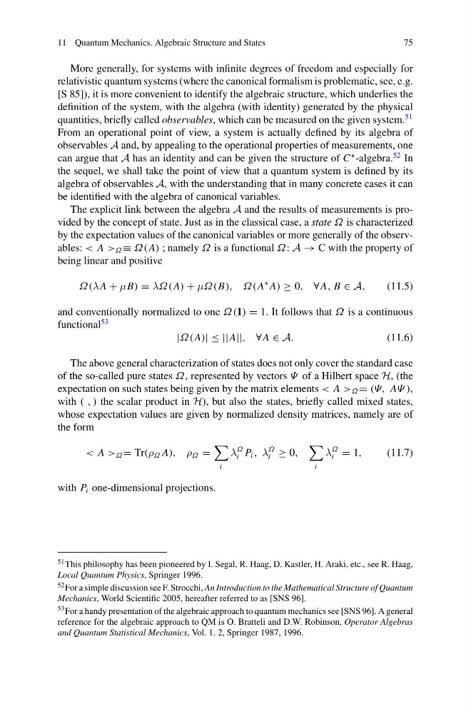
The explicit link between the algebra A and the results of measurements is provided by the concept of state. Just as in the classical case, a state Ω is characterized
by the expectation values of the canonical variables or more generally of the observables: < A > Ω ≡ Ω(A) ; namely Ω is a functional Ω: A → C with the property of
being linear and positive
Ω(λ A + μB) = λΩ(A) + μΩ(B), Ω(A
∗ A) ≥ 0, ∀A, B ∈ A,
(11.5)
and conventionally normalized to one Ω(1) = 1. It follows that Ω is a continuous
functional
53
|Ω(A)| ≤ ||A||, ∀A ∈ A.
(11.6)
The above general characterization of states does not only cover the standard case
of the so-called pure states Ω, represented by vectors Ψ of a Hilbert space H, (the
expectation on such states being given by the matrix elements < A > Ω = (Ψ, AΨ ),
with ( , ) the scalar product in H), but also the states, briefly called mixed states,
whose expectation values are given by normalized density matrices, namely are of
the form
< A > Ω = Tr(ρ Ω A), ρ Ω =
i
λ
Ω
i P i , λ
Ω
i ≥ 0,
i
λ
Ω
i = 1,
(11.7)
with P i one-dimensional projections.
51 This philosophy has been pioneered by I. Segal, R. Haag, D. Kastler, H. Araki, etc., see R. Haag,
Local Quantum Physics, Springer 1996.
52 For a simple discussion see F. Strocchi, An Introduction to the Mathematical Structure of Quantum
Mechanics, World Scientific 2005, hereafter referred to as [SNS 96].
53 For a handy presentation of the algebraic approach to quantum mechanics see [SNS 96]. A general
reference for the algebraic approach to QM is O. Bratteli and D.W. Robinson, Operator Algebras
and Quantum Statistical Mechanics, Vol. 1, 2, Springer 1987, 1996.
75
More generally, for systems with infinite degrees of freedom and especially for
relativistic quantum systems (where the canonical formalism is problematic, see, e.g.
[S 85]), it is more convenient to identify the algebraic structure, which underlies the
definition of the system, with the algebra (with identity) generated by the physical
quantities, briefly called observables, which can be measured on the given system.
51
From an operational point of view, a system is actually defined by its algebra of
observables A and, by appealing to the operational properties of measurements, one
can argue that A has an identity and can be given the structure of C
∗ -algebra.
52 In
the sequel, we shall take the point of view that a quantum system is defined by its
algebra of observables A, with the understanding that in many concrete cases it can
be identified with the algebra of canonical variables.
The explicit link between the algebra A and the results of measurements is provided by the concept of state. Just as in the classical case, a state Ω is characterized
by the expectation values of the canonical variables or more generally of the observables: < A > Ω ≡ Ω(A) ; namely Ω is a functional Ω: A → C with the property of
being linear and positive
Ω(λ A + μB) = λΩ(A) + μΩ(B), Ω(A
∗ A) ≥ 0, ∀A, B ∈ A,
(11.5)
and conventionally normalized to one Ω(1) = 1. It follows that Ω is a continuous
functional
53
|Ω(A)| ≤ ||A||, ∀A ∈ A.
(11.6)
The above general characterization of states does not only cover the standard case
of the so-called pure states Ω, represented by vectors Ψ of a Hilbert space H, (the
expectation on such states being given by the matrix elements < A > Ω = (Ψ, AΨ ),
with ( , ) the scalar product in H), but also the states, briefly called mixed states,
whose expectation values are given by normalized density matrices, namely are of
the form
< A > Ω = Tr(ρ Ω A), ρ Ω =
i
λ
Ω
i P i , λ
Ω
i ≥ 0,
i
λ
Ω
i = 1,
(11.7)
with P i one-dimensional projections.
51 This philosophy has been pioneered by I. Segal, R. Haag, D. Kastler, H. Araki, etc., see R. Haag,
Local Quantum Physics, Springer 1996.
52 For a simple discussion see F. Strocchi, An Introduction to the Mathematical Structure of Quantum
Mechanics, World Scientific 2005, hereafter referred to as [SNS 96].
53 For a handy presentation of the algebraic approach to quantum mechanics see [SNS 96]. A general
reference for the algebraic approach to QM is O. Bratteli and D.W. Robinson, Operator Algebras
and Quantum Statistical Mechanics, Vol. 1, 2, Springer 1987, 1996.