

5 Stable Structures, Hilbert Sectors, Phases
23
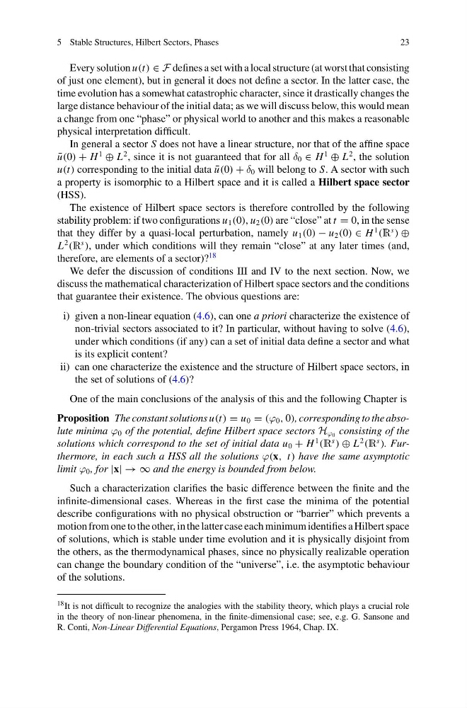
Every solution u(t) ∈ F defines a set with a local structure (at worst that consisting
of just one element), but in general it does not define a sector. In the latter case, the
time evolution has a somewhat catastrophic character, since it drastically changes the
large distance behaviour of the initial data; as we will discuss below, this would mean
a change from one “phase” or physical world to another and this makes a reasonable
physical interpretation difficult.
In general a sector S does not have a linear structure, nor that of the affine space
¯
u(0) + H
1
⊕ L
2 , since it is not guaranteed that for all δ 0 ∈ H
1
⊕ L
2 , the solution
u(t) corresponding to the initial data ¯
u(0) + δ 0 will belong to S. A sector with such
a property is isomorphic to a Hilbert space and it is called a Hilbert space sector
(HSS).
The existence of Hilbert space sectors is therefore controlled by the following
stability problem: if two configurations u 1 (0), u 2 (0) are “close” at t = 0, in the sense
that they differ by a quasi-local perturbation, namely u 1 (0) − u 2 (0) ∈ H
1
(R
s
) ⊕
L
2
(R
s
), under which conditions will they remain “close” at any later times (and,
therefore, are elements of a sector)?
18
We defer the discussion of conditions III and IV to the next section. Now, we
discuss the mathematical characterization of Hilbert space sectors and the conditions
that guarantee their existence. The obvious questions are:
i) given a non-linear equation (4.6), can one a priori characterize the existence of
non-trivial sectors associated to it? In particular, without having to solve (4.6),
under which conditions (if any) can a set of initial data define a sector and what
is its explicit content?
ii) can one characterize the existence and the structure of Hilbert space sectors, in
the set of solutions of (4.6)?
One of the main conclusions of the analysis of this and the following Chapter is
Proposition The constant solutions u(t) = u 0 = (ϕ 0 , 0), corresponding to the absolute minima ϕ 0 of the potential, define Hilbert space sectors H ϕ 0 consisting of the
solutions which correspond to the set of initial data u 0 + H
1
(R
s
) ⊕ L
2
(R
s
). Furthermore, in each such a HSS all the solutions ϕ(x, t) have the same asymptotic
limit ϕ 0 , for |x| → ∞ and the energy is bounded from below.
Such a characterization clarifies the basic difference between the finite and the
infinite-dimensional cases. Whereas in the first case the minima of the potential
describe configurations with no physical obstruction or “barrier” which prevents a
motion from one to the other, in the latter case each minimum identifies a Hilbert space
of solutions, which is stable under time evolution and it is physically disjoint from
the others, as the thermodynamical phases, since no physically realizable operation
can change the boundary condition of the “universe”, i.e. the asymptotic behaviour
of the solutions.
18 It is not difficult to recognize the analogies with the stability theory, which plays a crucial role
in the theory of non-linear phenomena, in the finite-dimensional case; see, e.g. G. Sansone and
R. Conti, Non-Linear Differential Equations, Pergamon Press 1964, Chap. IX.
23
Every solution u(t) ∈ F defines a set with a local structure (at worst that consisting
of just one element), but in general it does not define a sector. In the latter case, the
time evolution has a somewhat catastrophic character, since it drastically changes the
large distance behaviour of the initial data; as we will discuss below, this would mean
a change from one “phase” or physical world to another and this makes a reasonable
physical interpretation difficult.
In general a sector S does not have a linear structure, nor that of the affine space
¯
u(0) + H
1
⊕ L
2 , since it is not guaranteed that for all δ 0 ∈ H
1
⊕ L
2 , the solution
u(t) corresponding to the initial data ¯
u(0) + δ 0 will belong to S. A sector with such
a property is isomorphic to a Hilbert space and it is called a Hilbert space sector
(HSS).
The existence of Hilbert space sectors is therefore controlled by the following
stability problem: if two configurations u 1 (0), u 2 (0) are “close” at t = 0, in the sense
that they differ by a quasi-local perturbation, namely u 1 (0) − u 2 (0) ∈ H
1
(R
s
) ⊕
L
2
(R
s
), under which conditions will they remain “close” at any later times (and,
therefore, are elements of a sector)?
18
We defer the discussion of conditions III and IV to the next section. Now, we
discuss the mathematical characterization of Hilbert space sectors and the conditions
that guarantee their existence. The obvious questions are:
i) given a non-linear equation (4.6), can one a priori characterize the existence of
non-trivial sectors associated to it? In particular, without having to solve (4.6),
under which conditions (if any) can a set of initial data define a sector and what
is its explicit content?
ii) can one characterize the existence and the structure of Hilbert space sectors, in
the set of solutions of (4.6)?
One of the main conclusions of the analysis of this and the following Chapter is
Proposition The constant solutions u(t) = u 0 = (ϕ 0 , 0), corresponding to the absolute minima ϕ 0 of the potential, define Hilbert space sectors H ϕ 0 consisting of the
solutions which correspond to the set of initial data u 0 + H
1
(R
s
) ⊕ L
2
(R
s
). Furthermore, in each such a HSS all the solutions ϕ(x, t) have the same asymptotic
limit ϕ 0 , for |x| → ∞ and the energy is bounded from below.
Such a characterization clarifies the basic difference between the finite and the
infinite-dimensional cases. Whereas in the first case the minima of the potential
describe configurations with no physical obstruction or “barrier” which prevents a
motion from one to the other, in the latter case each minimum identifies a Hilbert space
of solutions, which is stable under time evolution and it is physically disjoint from
the others, as the thermodynamical phases, since no physically realizable operation
can change the boundary condition of the “universe”, i.e. the asymptotic behaviour
of the solutions.
18 It is not difficult to recognize the analogies with the stability theory, which plays a crucial role
in the theory of non-linear phenomena, in the finite-dimensional case; see, e.g. G. Sansone and
R. Conti, Non-Linear Differential Equations, Pergamon Press 1964, Chap. IX.