

246
Appendix C: Anderson Model of Superconductivity
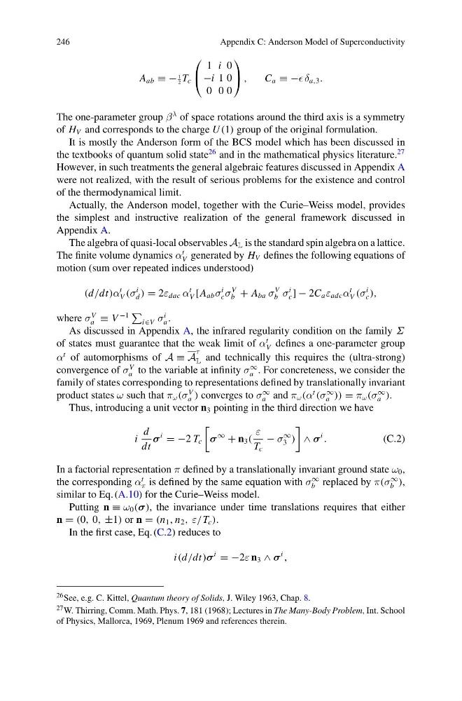
A ab ≡ −
1
2 T c
⎛
⎝
1 i 0
−i 1 0
0 0 0
⎞
⎠ ,
C a ≡ − δ a,3 .
The one-parameter group β
λ of space rotations around the third axis is a symmetry
of H V and corresponds to the charge U (1) group of the original formulation.
It is mostly the Anderson form of the BCS model which has been discussed in
the textbooks of quantum solid state
26 and in the mathematical physics literature.
27
However, in such treatments the general algebraic features discussed in Appendix A
were not realized, with the result of serious problems for the existence and control
of the thermodynamical limit.
Actually, the Anderson model, together with the Curie–Weiss model, provides
the simplest and instructive realization of the general framework discussed in
Appendix A.
The algebra of quasi-local observables A L is the standard spin algebra on a lattice.
The finite volume dynamics α
t
V generated by H V defines the following equations of
motion (sum over repeated indices understood)
(d/dt)α
t
V (σ
i
d ) = 2ε dac α
t
V [A ab σ
i
c σ
V
b + A ba σ
V
b σ
i
c ] − 2C a ε adc α
t
V (σ
i
c ),
where σ
V
a ≡ V
−1
i∈V σ
i
a .
As discussed in Appendix A, the infrared regularity condition on the family Σ
of states must guarantee that the weak limit of α
t
V defines a one-parameter group
α
t of automorphisms of A ≡ A
τ
L and technically this requires the (ultra-strong)
convergence of σ
V
a to the variable at infinity σ
∞
a . For concreteness, we consider the
family of states corresponding to representations defined by translationally invariant
product states ω such that π ω (σ
V
a ) converges to σ
∞
a and π ω (α
t
(σ
∞
a )) = π ω (σ
∞
a ).
Thus, introducing a unit vector n 3 pointing in the third direction we have
i
d
dt
σ
i
= −2 T c
σ
∞
+ n 3 (
ε
T c
− σ
∞
3 )
∧ σ
i
.
(C.2)
In a factorial representation π defined by a translationally invariant ground state ω 0 ,
the corresponding α
t
π is defined by the same equation with σ
∞
b replaced by π(σ
∞
b ),
similar to Eq. (A.10) for the Curie–Weiss model.
Putting n ≡ ω 0 (σ), the invariance under time translations requires that either
n = (0, 0, ±1) or n = (n 1 , n 2 , ε/T c ).
In the first case, Eq. (C.2) reduces to
i(d/dt)σ
i
= −2ε n 3 ∧ σ
i
,
26 See, e.g. C. Kittel, Quantum theory of Solids, J. Wiley 1963, Chap. 8.
27 W. Thirring, Comm. Math. Phys. 7, 181 (1968); Lectures in The Many-Body Problem, Int. School
of Physics, Mallorca, 1969, Plenum 1969 and references therein.
Appendix C: Anderson Model of Superconductivity
A ab ≡ −
1
2 T c
⎛
⎝
1 i 0
−i 1 0
0 0 0
⎞
⎠ ,
C a ≡ − δ a,3 .
The one-parameter group β
λ of space rotations around the third axis is a symmetry
of H V and corresponds to the charge U (1) group of the original formulation.
It is mostly the Anderson form of the BCS model which has been discussed in
the textbooks of quantum solid state
26 and in the mathematical physics literature.
27
However, in such treatments the general algebraic features discussed in Appendix A
were not realized, with the result of serious problems for the existence and control
of the thermodynamical limit.
Actually, the Anderson model, together with the Curie–Weiss model, provides
the simplest and instructive realization of the general framework discussed in
Appendix A.
The algebra of quasi-local observables A L is the standard spin algebra on a lattice.
The finite volume dynamics α
t
V generated by H V defines the following equations of
motion (sum over repeated indices understood)
(d/dt)α
t
V (σ
i
d ) = 2ε dac α
t
V [A ab σ
i
c σ
V
b + A ba σ
V
b σ
i
c ] − 2C a ε adc α
t
V (σ
i
c ),
where σ
V
a ≡ V
−1
i∈V σ
i
a .
As discussed in Appendix A, the infrared regularity condition on the family Σ
of states must guarantee that the weak limit of α
t
V defines a one-parameter group
α
t of automorphisms of A ≡ A
τ
L and technically this requires the (ultra-strong)
convergence of σ
V
a to the variable at infinity σ
∞
a . For concreteness, we consider the
family of states corresponding to representations defined by translationally invariant
product states ω such that π ω (σ
V
a ) converges to σ
∞
a and π ω (α
t
(σ
∞
a )) = π ω (σ
∞
a ).
Thus, introducing a unit vector n 3 pointing in the third direction we have
i
d
dt
σ
i
= −2 T c
σ
∞
+ n 3 (
ε
T c
− σ
∞
3 )
∧ σ
i
.
(C.2)
In a factorial representation π defined by a translationally invariant ground state ω 0 ,
the corresponding α
t
π is defined by the same equation with σ
∞
b replaced by π(σ
∞
b ),
similar to Eq. (A.10) for the Curie–Weiss model.
Putting n ≡ ω 0 (σ), the invariance under time translations requires that either
n = (0, 0, ±1) or n = (n 1 , n 2 , ε/T c ).
In the first case, Eq. (C.2) reduces to
i(d/dt)σ
i
= −2ε n 3 ∧ σ
i
,
26 See, e.g. C. Kittel, Quantum theory of Solids, J. Wiley 1963, Chap. 8.
27 W. Thirring, Comm. Math. Phys. 7, 181 (1968); Lectures in The Many-Body Problem, Int. School
of Physics, Mallorca, 1969, Plenum 1969 and references therein.