

Appendix A: Long Range Dynamics and Vacuum Seizing
231
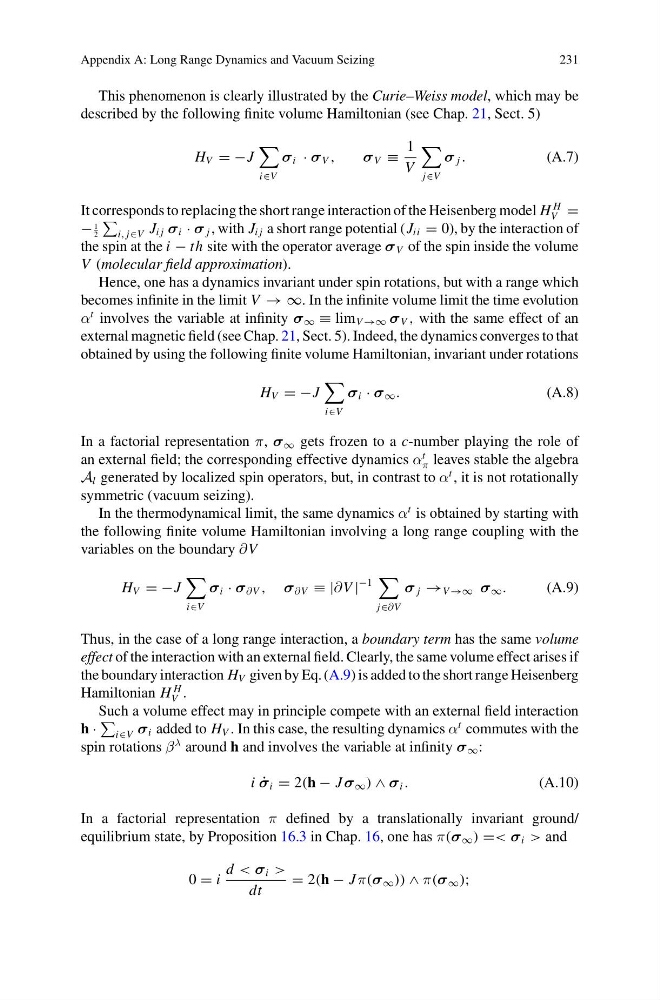
This phenomenon is clearly illustrated by the Curie–Weiss model, which may be
described by the following finite volume Hamiltonian (see Chap. 21, Sect. 5)
H V = −J
i∈V
σ i · σ V ,
σ V ≡
1
V
j∈V
σ j .
(A.7)
It corresponds to replacing the short range interaction of the Heisenberg model H
H
V =
−
1
2
i, j∈V J i j σ i · σ j , with J i j a short range potential (J ii = 0), by the interaction of
the spin at the i − th site with the operator average σ V of the spin inside the volume
V (molecular field approximation).
Hence, one has a dynamics invariant under spin rotations, but with a range which
becomes infinite in the limit V → ∞. In the infinite volume limit the time evolution
α
t involves the variable at infinity σ ∞ ≡ lim V →∞ σ V , with the same effect of an
external magnetic field (see Chap. 21, Sect. 5). Indeed, the dynamics converges to that
obtained by using the following finite volume Hamiltonian, invariant under rotations
H V = −J
i∈V
σ i · σ ∞ .
(A.8)
In a factorial representation π, σ ∞ gets frozen to a c-number playing the role of
an external field; the corresponding effective dynamics α
t
π leaves stable the algebra
A l generated by localized spin operators, but, in contrast to α
t , it is not rotationally
symmetric (vacuum seizing).
In the thermodynamical limit, the same dynamics α
t is obtained by starting with
the following finite volume Hamiltonian involving a long range coupling with the
variables on the boundary ∂V
H V = −J
i∈V
σ i · σ ∂V , σ ∂V ≡ |∂V |
−1
j∈∂V
σ j → V →∞ σ ∞ .
(A.9)
Thus, in the case of a long range interaction, a boundary term has the same volume
effect of the interaction with an external field. Clearly, the same volume effect arises if
the boundary interaction H V given by Eq. (A.9) is added to the short range Heisenberg
Hamiltonian H
H
V .
Such a volume effect may in principle compete with an external field interaction
h ·
i∈V σ i added to H V . In this case, the resulting dynamics α
t commutes with the
spin rotations β
λ around h and involves the variable at infinity σ ∞ :
i ˙
σ i = 2(h − J σ ∞ ) ∧ σ i .
(A.10)
In a factorial representation π defined by a translationally invariant ground/
equilibrium state, by Proposition 16.3 in Chap. 16, one has π(σ ∞ ) =< σ i > and
0 = i
d < σ i >
dt
= 2(h − J π(σ ∞ )) ∧ π(σ ∞ );
231
This phenomenon is clearly illustrated by the Curie–Weiss model, which may be
described by the following finite volume Hamiltonian (see Chap. 21, Sect. 5)
H V = −J
i∈V
σ i · σ V ,
σ V ≡
1
V
j∈V
σ j .
(A.7)
It corresponds to replacing the short range interaction of the Heisenberg model H
H
V =
−
1
2
i, j∈V J i j σ i · σ j , with J i j a short range potential (J ii = 0), by the interaction of
the spin at the i − th site with the operator average σ V of the spin inside the volume
V (molecular field approximation).
Hence, one has a dynamics invariant under spin rotations, but with a range which
becomes infinite in the limit V → ∞. In the infinite volume limit the time evolution
α
t involves the variable at infinity σ ∞ ≡ lim V →∞ σ V , with the same effect of an
external magnetic field (see Chap. 21, Sect. 5). Indeed, the dynamics converges to that
obtained by using the following finite volume Hamiltonian, invariant under rotations
H V = −J
i∈V
σ i · σ ∞ .
(A.8)
In a factorial representation π, σ ∞ gets frozen to a c-number playing the role of
an external field; the corresponding effective dynamics α
t
π leaves stable the algebra
A l generated by localized spin operators, but, in contrast to α
t , it is not rotationally
symmetric (vacuum seizing).
In the thermodynamical limit, the same dynamics α
t is obtained by starting with
the following finite volume Hamiltonian involving a long range coupling with the
variables on the boundary ∂V
H V = −J
i∈V
σ i · σ ∂V , σ ∂V ≡ |∂V |
−1
j∈∂V
σ j → V →∞ σ ∞ .
(A.9)
Thus, in the case of a long range interaction, a boundary term has the same volume
effect of the interaction with an external field. Clearly, the same volume effect arises if
the boundary interaction H V given by Eq. (A.9) is added to the short range Heisenberg
Hamiltonian H
H
V .
Such a volume effect may in principle compete with an external field interaction
h ·
i∈V σ i added to H V . In this case, the resulting dynamics α
t commutes with the
spin rotations β
λ around h and involves the variable at infinity σ ∞ :
i ˙
σ i = 2(h − J σ ∞ ) ∧ σ i .
(A.10)
In a factorial representation π defined by a translationally invariant ground/
equilibrium state, by Proposition 16.3 in Chap. 16, one has π(σ ∞ ) =< σ i > and
0 = i
d < σ i >
dt
= 2(h − J π(σ ∞ )) ∧ π(σ ∞ );