

196
27 The Goldstone Theorem for Relativistic Local Fields
of the role of locality and its failure in positive gauges establishes a strong bridge
between gauge quantum field theories and many body theories like superconductivity
and Coulomb systems (see discussion in Sect. 25.2 and in Chap. 29).
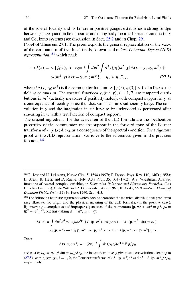
Proof of Theorem 27.1. The proof exploits the general representation of the v.e.v.
of the commutator of two local fields, known as the Jost–Lehmann–Dyson (JLD)
representation,
181 which reads
− i J (x) ≡ < [ j 0 (x), A] > 0 = i
dm
2
d
3 y{ρ 1 (m
2
, y))(x − y, x 0 ; m
2
) +
ρ 2 (m
2
, y) ˙
(x − y, x 0 ; m
2
)}, j 0 , A ∈ F loc ,
(27.5)
where i(x, x 0 ; m
2
) is the commutator function < [ϕ(x), ϕ(0)] > 0 of a free scalar
field ϕ of mass m. The spectral functions ρ i (m
2
, y), i = 1, 2, are tempered distributions in m
2 (actually measures if positivity holds), with compact support in y as
a consequence of locality, since the l.h.s. vanishes for x sufficiently large. The convolution in y and the integration in m
2 have to be understood as performed after
smearing in x, with a test function of compact support.
The crucial ingredients for the derivation of the JLD formula are the localization
properties of the commutator and the support in the forward cone of the Fourier
transform of < j 0 (x)A > 0 , as a consequence of the spectral condition. For a rigorous
proof of the JLD representation, we refer to the references given in the previous
footnote.
182
181 R. Jost and H. Lehmann, Nuovo Cim. 5, 1598 (1957); F. Dyson, Phys. Rev. 110, 1460 (1958);
H. Araki, K. Hepp and D. Ruelle, Helv. Acta Phys. 35, 164 (1962); A.S. Wightman, Analytic
functions of several complex variables, in Dispersion Relations and Elementary Particles, (Les
Houches Lectures), C. de Witt and R. Omnes eds., Wiley 1961; H. Araki, Mathematical Theory of
Quantum Fields, Oxford Univ. Press 1999, Sect. 4.5.
182 The following heuristic argument (which does not consider the technical distributional problems)
may illustrate the origin and the physical meaning of the JLD formula, (in the positive case).
By inserting a complete set of improper eigenstates of the momentum |p, m 2 >, m 2 ≡ p 2 , p 0 ≡
(p 2 + m 2 ) 1/2 , one has (taking A = A ∗ , j 0 = j ∗
0 )
−i J(x) =
dm
2 d
3 p/(2 p 0 )e
ip·x [J − (p, m
2 ) cos( p 0 x 0 ) − i J + (p, m
2 ) sin( p 0 x 0 )],
J ± (p, m
2 ) ≡< j 0 |p, m
2 >< p, m
2 |A > ± < A|p, m
2 >< p, m
2 | j 0 > .
Since
(x, x 0 ; m
2 ) = −(2π)
−3
sin( p 0 x 0 )e
ip·x d
3 p/ p 0
and cos( p 0 x 0 ) = p
−1
0 d sin( p 0 x 0 )/dx 0 , the integrations in d 3 p give rise to convolutions, leading to
(27.5), with ρ i (m 2 , y), i = 1, 2, the Fourier transforms of i J + (p, m 2 )/2 and of −J − (p, m 2 )/2 p 0 ,
respectively.
27 The Goldstone Theorem for Relativistic Local Fields
of the role of locality and its failure in positive gauges establishes a strong bridge
between gauge quantum field theories and many body theories like superconductivity
and Coulomb systems (see discussion in Sect. 25.2 and in Chap. 29).
Proof of Theorem 27.1. The proof exploits the general representation of the v.e.v.
of the commutator of two local fields, known as the Jost–Lehmann–Dyson (JLD)
representation,
181 which reads
− i J (x) ≡ < [ j 0 (x), A] > 0 = i
dm
2
d
3 y{ρ 1 (m
2
, y))(x − y, x 0 ; m
2
) +
ρ 2 (m
2
, y) ˙
(x − y, x 0 ; m
2
)}, j 0 , A ∈ F loc ,
(27.5)
where i(x, x 0 ; m
2
) is the commutator function < [ϕ(x), ϕ(0)] > 0 of a free scalar
field ϕ of mass m. The spectral functions ρ i (m
2
, y), i = 1, 2, are tempered distributions in m
2 (actually measures if positivity holds), with compact support in y as
a consequence of locality, since the l.h.s. vanishes for x sufficiently large. The convolution in y and the integration in m
2 have to be understood as performed after
smearing in x, with a test function of compact support.
The crucial ingredients for the derivation of the JLD formula are the localization
properties of the commutator and the support in the forward cone of the Fourier
transform of < j 0 (x)A > 0 , as a consequence of the spectral condition. For a rigorous
proof of the JLD representation, we refer to the references given in the previous
footnote.
182
181 R. Jost and H. Lehmann, Nuovo Cim. 5, 1598 (1957); F. Dyson, Phys. Rev. 110, 1460 (1958);
H. Araki, K. Hepp and D. Ruelle, Helv. Acta Phys. 35, 164 (1962); A.S. Wightman, Analytic
functions of several complex variables, in Dispersion Relations and Elementary Particles, (Les
Houches Lectures), C. de Witt and R. Omnes eds., Wiley 1961; H. Araki, Mathematical Theory of
Quantum Fields, Oxford Univ. Press 1999, Sect. 4.5.
182 The following heuristic argument (which does not consider the technical distributional problems)
may illustrate the origin and the physical meaning of the JLD formula, (in the positive case).
By inserting a complete set of improper eigenstates of the momentum |p, m 2 >, m 2 ≡ p 2 , p 0 ≡
(p 2 + m 2 ) 1/2 , one has (taking A = A ∗ , j 0 = j ∗
0 )
−i J(x) =
dm
2 d
3 p/(2 p 0 )e
ip·x [J − (p, m
2 ) cos( p 0 x 0 ) − i J + (p, m
2 ) sin( p 0 x 0 )],
J ± (p, m
2 ) ≡< j 0 |p, m
2 >< p, m
2 |A > ± < A|p, m
2 >< p, m
2 | j 0 > .
Since
(x, x 0 ; m
2 ) = −(2π)
−3
sin( p 0 x 0 )e
ip·x d
3 p/ p 0
and cos( p 0 x 0 ) = p
−1
0 d sin( p 0 x 0 )/dx 0 , the integrations in d 3 p give rise to convolutions, leading to
(27.5), with ρ i (m 2 , y), i = 1, 2, the Fourier transforms of i J + (p, m 2 )/2 and of −J − (p, m 2 )/2 p 0 ,
respectively.