

38
2 Experimental Methods for Determination of Nucleation Rates
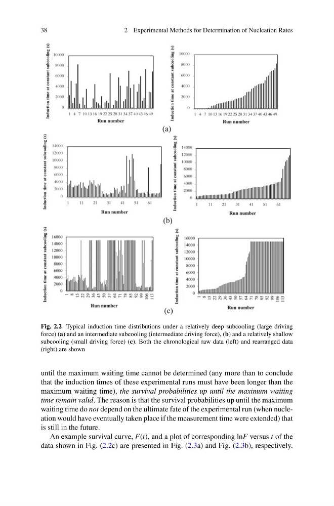
Fig. 2.2 Typical induction time distributions under a relatively deep subcooling (large driving
force) (a) and an intermediate subcooling (intermediate driving force), (b) and a relatively shallow
subcooling (small driving force) (c). Both the chronological raw data (left) and rearranged data
(right) are shown
until the maximum waiting time cannot be determined (any more than to conclude
that the induction times of these experimental runs must have been longer than the
maximum waiting time), the survival probabilities up until the maximum waiting
time remain valid. The reason is that the survival probabilities up until the maximum
waiting time do not depend on the ultimate fate of the experimental run (when nucleation would have eventually taken place if the measurement time were extended) that
is still in the future.
An example survival curve, F(t), and a plot of corresponding lnF versus t of the
data shown in Fig. (2.2c) are presented in Fig. (2.3a) and Fig. (2.3b), respectively.
2 Experimental Methods for Determination of Nucleation Rates
Fig. 2.2 Typical induction time distributions under a relatively deep subcooling (large driving
force) (a) and an intermediate subcooling (intermediate driving force), (b) and a relatively shallow
subcooling (small driving force) (c). Both the chronological raw data (left) and rearranged data
(right) are shown
until the maximum waiting time cannot be determined (any more than to conclude
that the induction times of these experimental runs must have been longer than the
maximum waiting time), the survival probabilities up until the maximum waiting
time remain valid. The reason is that the survival probabilities up until the maximum
waiting time do not depend on the ultimate fate of the experimental run (when nucleation would have eventually taken place if the measurement time were extended) that
is still in the future.
An example survival curve, F(t), and a plot of corresponding lnF versus t of the
data shown in Fig. (2.2c) are presented in Fig. (2.3a) and Fig. (2.3b), respectively.