

10 A Novel High-Efficiency Keyhole Tungsten Inert Gas …
341
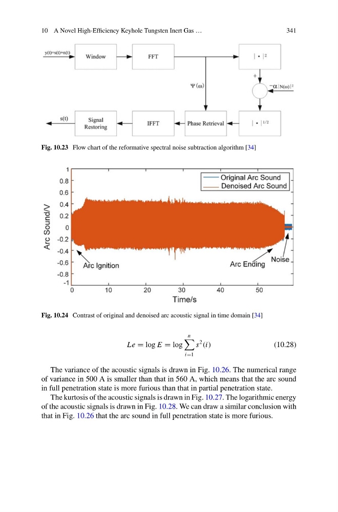
Fig. 10.23 Flow chart of the reformative spectral noise subtraction algorithm [34]
Fig. 10.24 Contrast of original and denoised arc acoustic signal in time domain [34]
Le = log E = log
n
i=1
s
2
(i)
(10.28)
The variance of the acoustic signals is drawn in Fig. 10.26. The numerical range
of variance in 500 A is smaller than that in 560 A, which means that the arc sound
in full penetration state is more furious than that in partial penetration state.
The kurtosis of the acoustic signals is drawn in Fig. 10.27. The logarithmic energy
of the acoustic signals is drawn in Fig. 10.28. We can draw a similar conclusion with
that in Fig. 10.26 that the arc sound in full penetration state is more furious.
341
Fig. 10.23 Flow chart of the reformative spectral noise subtraction algorithm [34]
Fig. 10.24 Contrast of original and denoised arc acoustic signal in time domain [34]
Le = log E = log
n
i=1
s
2
(i)
(10.28)
The variance of the acoustic signals is drawn in Fig. 10.26. The numerical range
of variance in 500 A is smaller than that in 560 A, which means that the arc sound
in full penetration state is more furious than that in partial penetration state.
The kurtosis of the acoustic signals is drawn in Fig. 10.27. The logarithmic energy
of the acoustic signals is drawn in Fig. 10.28. We can draw a similar conclusion with
that in Fig. 10.26 that the arc sound in full penetration state is more furious.