

8 Industry 4.0 in Welding
291
predicts the tensile strength of the weld in real time. This covers a part of the objective
of this case study.
For the second part of the objective, i.e. online control of the weld quality, the data
processing script is fed with a reference tensile strength value. This reference value
is based upon the application for which the weld is being fabricated. A decision box
compares the outcome of the ML(1) with this reference value. The reference value
would come from the PQR of the FSW joint, the corresponding joining and other
parameters can be found from the WPS. Thus, during the welding, if any defect
is produced, then the reference tensile strength value cannot be retained. Hence,
the decision box comparison is justified. When the predicted value is more than
the reference value, this indicates that the weld joint is proper and the procedure is
maintained. In this scenario, the parameters remain unchanged (indicated as “No,
deviation” in Fig. 8.16). If the predicted value is lower than the reference value
(indicated as “Yes, deviation” in Fig. 8.16), the corresponding batch of data is sent
to another ML model, ML(2). The inputs to the ML(2) were also the D1 coefficients
of force, but the outputs were rotational speed and welding speed. These predicted
parameters are sent as feedback to the FSW machine.
Thus, the cloud server consists of the models, ML(1) and ML(2), data processing
script, database, and this combination represents the cyber component. They analyse
the data acquired from the physical FSW machine, and control the machine based
on certain decisions. This accomplishes the definition of CPS. The trained models
were plugged in the developed architecture for real-time control.
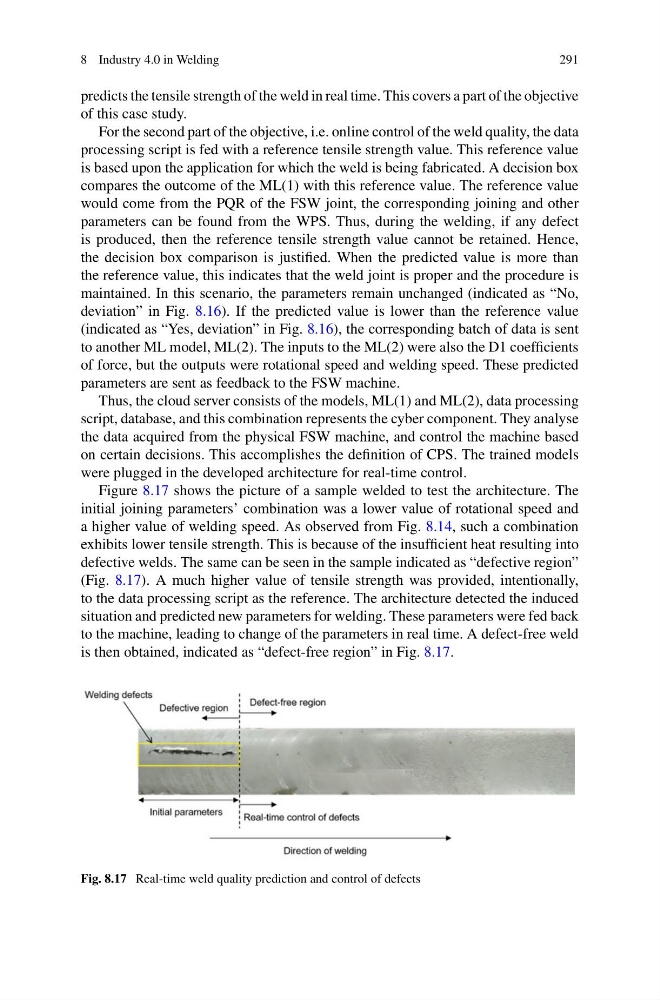
Figure 8.17 shows the picture of a sample welded to test the architecture. The
initial joining parameters’ combination was a lower value of rotational speed and
a higher value of welding speed. As observed from Fig. 8.14, such a combination
exhibits lower tensile strength. This is because of the insufficient heat resulting into
defective welds. The same can be seen in the sample indicated as “defective region”
(Fig. 8.17). A much higher value of tensile strength was provided, intentionally,
to the data processing script as the reference. The architecture detected the induced
situation and predicted new parameters for welding. These parameters were fed back
to the machine, leading to change of the parameters in real time. A defect-free weld
is then obtained, indicated as “defect-free region” in Fig. 8.17.
Fig. 8.17 Real-time weld quality prediction and control of defects
291
predicts the tensile strength of the weld in real time. This covers a part of the objective
of this case study.
For the second part of the objective, i.e. online control of the weld quality, the data
processing script is fed with a reference tensile strength value. This reference value
is based upon the application for which the weld is being fabricated. A decision box
compares the outcome of the ML(1) with this reference value. The reference value
would come from the PQR of the FSW joint, the corresponding joining and other
parameters can be found from the WPS. Thus, during the welding, if any defect
is produced, then the reference tensile strength value cannot be retained. Hence,
the decision box comparison is justified. When the predicted value is more than
the reference value, this indicates that the weld joint is proper and the procedure is
maintained. In this scenario, the parameters remain unchanged (indicated as “No,
deviation” in Fig. 8.16). If the predicted value is lower than the reference value
(indicated as “Yes, deviation” in Fig. 8.16), the corresponding batch of data is sent
to another ML model, ML(2). The inputs to the ML(2) were also the D1 coefficients
of force, but the outputs were rotational speed and welding speed. These predicted
parameters are sent as feedback to the FSW machine.
Thus, the cloud server consists of the models, ML(1) and ML(2), data processing
script, database, and this combination represents the cyber component. They analyse
the data acquired from the physical FSW machine, and control the machine based
on certain decisions. This accomplishes the definition of CPS. The trained models
were plugged in the developed architecture for real-time control.
Figure 8.17 shows the picture of a sample welded to test the architecture. The
initial joining parameters’ combination was a lower value of rotational speed and
a higher value of welding speed. As observed from Fig. 8.14, such a combination
exhibits lower tensile strength. This is because of the insufficient heat resulting into
defective welds. The same can be seen in the sample indicated as “defective region”
(Fig. 8.17). A much higher value of tensile strength was provided, intentionally,
to the data processing script as the reference. The architecture detected the induced
situation and predicted new parameters for welding. These parameters were fed back
to the machine, leading to change of the parameters in real time. A defect-free weld
is then obtained, indicated as “defect-free region” in Fig. 8.17.
Fig. 8.17 Real-time weld quality prediction and control of defects