

3 Modeling of Friction Stir Welding Processes
119
ρ ¨
u + c b ˙
u + k s u = F b ,
(3.93)
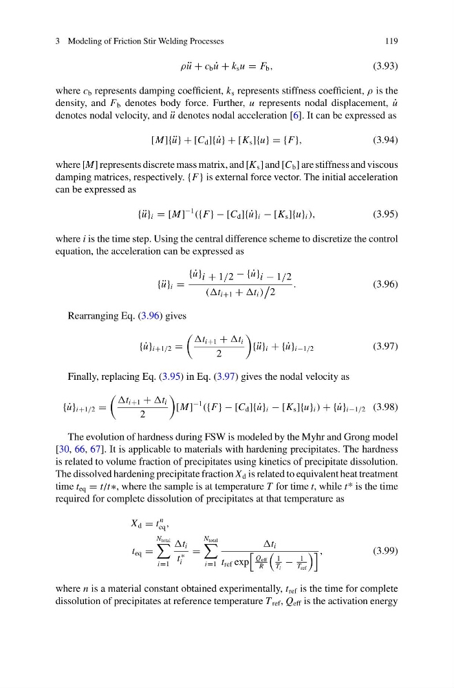
where c b represents damping coefficient, k s represents stiffness coefficient, ρ is the
density, and F b denotes body force. Further, u represents nodal displacement, ˙
u
denotes nodal velocity, and ¨
u denotes nodal acceleration [6]. It can be expressed as
[M]{ ¨
u} + [C d ]{ ˙
u} + [K s ]{u} = {F},
(3.94)
where [M] represents discrete mass matrix, and [K s ] and [C b ] are stiffness and viscous
damping matrices, respectively. {F} is external force vector. The initial acceleration
can be expressed as
{ ¨
u} i = [M]
−1
({F} − [C d ]{ ˙
u} i − [K s ]{u} i ),
(3.95)
where i is the time step. Using the central difference scheme to discretize the control
equation, the acceleration can be expressed as
{ ¨
u} i =
{ ˙
u} i + 1/2 − { ˙
u} i − 1/2
(t i+1 + t i )
2
.
(3.96)
Rearranging Eq. (3.96) gives
{ ˙
u} i+1/2 =
t i+1 + t i
2
{ ¨
u} i + { ˙
u} i−1/2
(3.97)
Finally, replacing Eq. (3.95) in Eq. (3.97) gives the nodal velocity as
{ ˙
u} i+1/2 =
t i+1 + t i
2
[M]
−1
({F} − [C d ]{ ˙
u} i − [K s ]{u} i ) + { ˙
u} i−1/2 (3.98)
The evolution of hardness during FSW is modeled by the Myhr and Grong model
[30, 66, 67]. It is applicable to materials with hardening precipitates. The hardness
is related to volume fraction of precipitates using kinetics of precipitate dissolution.
The dissolved hardening precipitate fraction X d is related to equivalent heat treatment
time t eq = t/t∗, where the sample is at temperature T for time t, while t* is the time
required for complete dissolution of precipitates at that temperature as
X d = t
n
eq ,
t eq =
N total
i=1
t i
t
∗
i
=
N total
i=1
t i
t ref exp
Q eff
R
1
T i
−
1
T ref
,
(3.99)
where n is a material constant obtained experimentally, t ref is the time for complete
dissolution of precipitates at reference temperature T ref , Q eff is the activation energy
119
ρ ¨
u + c b ˙
u + k s u = F b ,
(3.93)
where c b represents damping coefficient, k s represents stiffness coefficient, ρ is the
density, and F b denotes body force. Further, u represents nodal displacement, ˙
u
denotes nodal velocity, and ¨
u denotes nodal acceleration [6]. It can be expressed as
[M]{ ¨
u} + [C d ]{ ˙
u} + [K s ]{u} = {F},
(3.94)
where [M] represents discrete mass matrix, and [K s ] and [C b ] are stiffness and viscous
damping matrices, respectively. {F} is external force vector. The initial acceleration
can be expressed as
{ ¨
u} i = [M]
−1
({F} − [C d ]{ ˙
u} i − [K s ]{u} i ),
(3.95)
where i is the time step. Using the central difference scheme to discretize the control
equation, the acceleration can be expressed as
{ ¨
u} i =
{ ˙
u} i + 1/2 − { ˙
u} i − 1/2
(t i+1 + t i )
2
.
(3.96)
Rearranging Eq. (3.96) gives
{ ˙
u} i+1/2 =
t i+1 + t i
2
{ ¨
u} i + { ˙
u} i−1/2
(3.97)
Finally, replacing Eq. (3.95) in Eq. (3.97) gives the nodal velocity as
{ ˙
u} i+1/2 =
t i+1 + t i
2
[M]
−1
({F} − [C d ]{ ˙
u} i − [K s ]{u} i ) + { ˙
u} i−1/2 (3.98)
The evolution of hardness during FSW is modeled by the Myhr and Grong model
[30, 66, 67]. It is applicable to materials with hardening precipitates. The hardness
is related to volume fraction of precipitates using kinetics of precipitate dissolution.
The dissolved hardening precipitate fraction X d is related to equivalent heat treatment
time t eq = t/t∗, where the sample is at temperature T for time t, while t* is the time
required for complete dissolution of precipitates at that temperature as
X d = t
n
eq ,
t eq =
N total
i=1
t i
t
∗
i
=
N total
i=1
t i
t ref exp
Q eff
R
1
T i
−
1
T ref
,
(3.99)
where n is a material constant obtained experimentally, t ref is the time for complete
dissolution of precipitates at reference temperature T ref , Q eff is the activation energy