

3 Modeling of Friction Stir Welding Processes
115
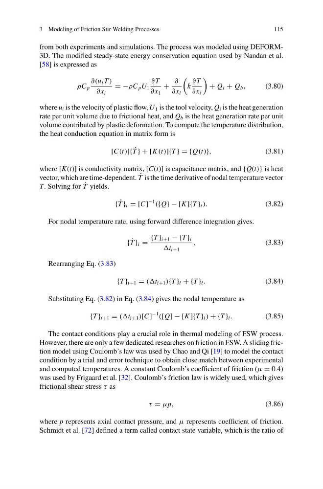
from both experiments and simulations. The process was modeled using DEFORM3D. The modified steady-state energy conservation equation used by Nandan et al.
[58] is expressed as
ρC p
∂(u i T )
∂ x i
= −ρC p U 1
∂ T
∂ x 1
+
∂
∂ x i
k
∂ T
∂ x i
+ Q i + Q b ,
(3.80)
where u i is the velocity of plastic flow, U 1 is the tool velocity, Q i is the heat generation
rate per unit volume due to frictional heat, and Q b is the heat generation rate per unit
volume contributed by plastic deformation. To compute the temperature distribution,
the heat conduction equation in matrix form is
[C(t)]{ ˙
T } + [K (t)]{T } = {Q(t)},
(3.81)
where [K(t)] is conductivity matrix, [C(t)] is capacitance matrix, and {Q(t)} is heat
vector, which are time-dependent. ˙
T is the time derivative of nodal temperature vector
T. Solving for ˙
T yields.
{ ˙
T } i = [C]
−1
({Q} − [K ]{T } i ).
(3.82)
For nodal temperature rate, using forward difference integration gives.
{ ˙
T } i =
{T } i+1 − {T } i
t i+1
,
(3.83)
Rearranging Eq. (3.83)
{T } i+1 = (t i+1 ){T } i + {T } i .
(3.84)
Substituting Eq. (3.82) in Eq. (3.84) gives the nodal temperature as
{T } i+1 = (t i+1 )[C]
−1
([Q] − [K ]{T } i ) + {T } i .
(3.85)
The contact conditions play a crucial role in thermal modeling of FSW process.
However, there are only a few dedicated researches on friction in FSW. A sliding friction model using Coulomb’s law was used by Chao and Qi [19] to model the contact
condition by a trial and error technique to obtain close match between experimental
and computed temperatures. A constant Coulomb’s coefficient of friction (μ = 0.4)
was used by Frigaard et al. [32]. Coulomb’s friction law is widely used, which gives
frictional shear stress τ as
τ = μp,
(3.86)
where p represents axial contact pressure, and μ represents coefficient of friction.
Schmidt et al. [72] defined a term called contact state variable, which is the ratio of
115
from both experiments and simulations. The process was modeled using DEFORM3D. The modified steady-state energy conservation equation used by Nandan et al.
[58] is expressed as
ρC p
∂(u i T )
∂ x i
= −ρC p U 1
∂ T
∂ x 1
+
∂
∂ x i
k
∂ T
∂ x i
+ Q i + Q b ,
(3.80)
where u i is the velocity of plastic flow, U 1 is the tool velocity, Q i is the heat generation
rate per unit volume due to frictional heat, and Q b is the heat generation rate per unit
volume contributed by plastic deformation. To compute the temperature distribution,
the heat conduction equation in matrix form is
[C(t)]{ ˙
T } + [K (t)]{T } = {Q(t)},
(3.81)
where [K(t)] is conductivity matrix, [C(t)] is capacitance matrix, and {Q(t)} is heat
vector, which are time-dependent. ˙
T is the time derivative of nodal temperature vector
T. Solving for ˙
T yields.
{ ˙
T } i = [C]
−1
({Q} − [K ]{T } i ).
(3.82)
For nodal temperature rate, using forward difference integration gives.
{ ˙
T } i =
{T } i+1 − {T } i
t i+1
,
(3.83)
Rearranging Eq. (3.83)
{T } i+1 = (t i+1 ){T } i + {T } i .
(3.84)
Substituting Eq. (3.82) in Eq. (3.84) gives the nodal temperature as
{T } i+1 = (t i+1 )[C]
−1
([Q] − [K ]{T } i ) + {T } i .
(3.85)
The contact conditions play a crucial role in thermal modeling of FSW process.
However, there are only a few dedicated researches on friction in FSW. A sliding friction model using Coulomb’s law was used by Chao and Qi [19] to model the contact
condition by a trial and error technique to obtain close match between experimental
and computed temperatures. A constant Coulomb’s coefficient of friction (μ = 0.4)
was used by Frigaard et al. [32]. Coulomb’s friction law is widely used, which gives
frictional shear stress τ as
τ = μp,
(3.86)
where p represents axial contact pressure, and μ represents coefficient of friction.
Schmidt et al. [72] defined a term called contact state variable, which is the ratio of