

3 Modeling of Friction Stir Welding Processes
97
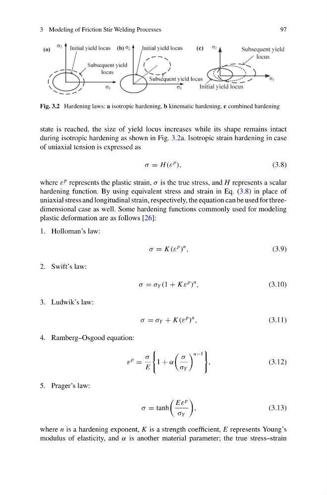
Fig. 3.2 Hardening laws: a isotropic hardening, b kinematic hardening, c combined hardening
state is reached, the size of yield locus increases while its shape remains intact
during isotropic hardening as shown in Fig. 3.2a. Isotropic strain hardening in case
of uniaxial tension is expressed as
σ = H (ε
p
),
(3.8)
where ε
p represents the plastic strain, σ is the true stress, and H represents a scalar
hardening function. By using equivalent stress and strain in Eq. (3.8) in place of
uniaxial stress and longitudinal strain, respectively, the equation can be used for threedimensional case as well. Some hardening functions commonly used for modeling
plastic deformation are as follows [26]:
1. Holloman’s law:
σ = K (ε
p
)
n
,
(3.9)
2. Swift’s law:
σ = σ Y (1 + K ε
p
)
n
,
(3.10)
3. Ludwik’s law:
σ = σ Y + K (ε
p
)
n
,
(3.11)
4. Ramberg–Osgood equation:
ε
p
=
σ
E
1 + α
σ
σ Y
n−1
,
(3.12)
5. Prager’s law:
σ = tanh
Eε
p
σ Y
,
(3.13)
where n is a hardening exponent, K is a strength coefficient, E represents Young’s
modulus of elasticity, and α is another material parameter; the true stress–strain
97
Fig. 3.2 Hardening laws: a isotropic hardening, b kinematic hardening, c combined hardening
state is reached, the size of yield locus increases while its shape remains intact
during isotropic hardening as shown in Fig. 3.2a. Isotropic strain hardening in case
of uniaxial tension is expressed as
σ = H (ε
p
),
(3.8)
where ε
p represents the plastic strain, σ is the true stress, and H represents a scalar
hardening function. By using equivalent stress and strain in Eq. (3.8) in place of
uniaxial stress and longitudinal strain, respectively, the equation can be used for threedimensional case as well. Some hardening functions commonly used for modeling
plastic deformation are as follows [26]:
1. Holloman’s law:
σ = K (ε
p
)
n
,
(3.9)
2. Swift’s law:
σ = σ Y (1 + K ε
p
)
n
,
(3.10)
3. Ludwik’s law:
σ = σ Y + K (ε
p
)
n
,
(3.11)
4. Ramberg–Osgood equation:
ε
p
=
σ
E
1 + α
σ
σ Y
n−1
,
(3.12)
5. Prager’s law:
σ = tanh
Eε
p
σ Y
,
(3.13)
where n is a hardening exponent, K is a strength coefficient, E represents Young’s
modulus of elasticity, and α is another material parameter; the true stress–strain