

plasma, which, in turn, controls the divertor performance. A straightforward way
from this problem would be reducing the time step in the iterations with Eqs. (8.1);
however, this is time-consuming and often impractical.
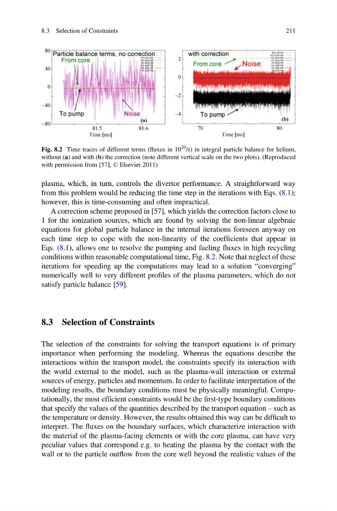
A correction scheme proposed in [57], which yields the correction factors close to
1 for the ionization sources, which are found by solving the non-linear algebraic
equations for global particle balance in the internal iterations foreseen anyway on
each time step to cope with the non-linearity of the coefficients that appear in
Eqs. (8.1), allows one to resolve the pumping and fueling fluxes in high recycling
conditions within reasonable computational time, Fig. 8.2. Note that neglect of these
iterations for speeding up the computations may lead to a solution “converging”
numerically well to very different profiles of the plasma parameters, which do not
satisfy particle balance [59].
8.3 Selection of Constraints
The selection of the constraints for solving the transport equations is of primary
importance when performing the modeling. Whereas the equations describe the
interactions within the transport model, the constraints specify its interaction with
the world external to the model, such as the plasma-wall interaction or external
sources of energy, particles and momentum. In order to facilitate interpretation of the
modeling results, the boundary conditions must be physically meaningful. Computationally, the most efficient constraints would be the first-type boundary conditions
that specify the values of the quantities described by the transport equation – such as
the temperature or density. However, the results obtained this way can be difficult to
interpret. The fluxes on the boundary surfaces, which characterize interaction with
the material of the plasma-facing elements or with the core plasma, can have very
peculiar values that correspond e.g. to heating the plasma by the contact with the
wall or to the particle outflow from the core well beyond the realistic values of the
Fig. 8.2 Time traces of different terms (fluxes in 10
20
/s) in integral particle balance for helium,
without (a) and with (b) the correction (note different vertical scale on the two plots). (Reproduced
with permission from [57], © Elsevier 2011)
8.3 Selection of Constraints
211
from this problem would be reducing the time step in the iterations with Eqs. (8.1);
however, this is time-consuming and often impractical.
A correction scheme proposed in [57], which yields the correction factors close to
1 for the ionization sources, which are found by solving the non-linear algebraic
equations for global particle balance in the internal iterations foreseen anyway on
each time step to cope with the non-linearity of the coefficients that appear in
Eqs. (8.1), allows one to resolve the pumping and fueling fluxes in high recycling
conditions within reasonable computational time, Fig. 8.2. Note that neglect of these
iterations for speeding up the computations may lead to a solution “converging”
numerically well to very different profiles of the plasma parameters, which do not
satisfy particle balance [59].
8.3 Selection of Constraints
The selection of the constraints for solving the transport equations is of primary
importance when performing the modeling. Whereas the equations describe the
interactions within the transport model, the constraints specify its interaction with
the world external to the model, such as the plasma-wall interaction or external
sources of energy, particles and momentum. In order to facilitate interpretation of the
modeling results, the boundary conditions must be physically meaningful. Computationally, the most efficient constraints would be the first-type boundary conditions
that specify the values of the quantities described by the transport equation – such as
the temperature or density. However, the results obtained this way can be difficult to
interpret. The fluxes on the boundary surfaces, which characterize interaction with
the material of the plasma-facing elements or with the core plasma, can have very
peculiar values that correspond e.g. to heating the plasma by the contact with the
wall or to the particle outflow from the core well beyond the realistic values of the
Fig. 8.2 Time traces of different terms (fluxes in 10
20
/s) in integral particle balance for helium,
without (a) and with (b) the correction (note different vertical scale on the two plots). (Reproduced
with permission from [57], © Elsevier 2011)
8.3 Selection of Constraints
211