

fluid approximation become (e.g. see [13]) λ C /L k and
ffiffiffiffiffiffiffiffi
λ C ρ
p
=L ⊥ , where ρ ¼
ffiffiffiffiffiffiffiffiffi ffi
T=m
p
=Ω B is the particle Larmor radius whereas L k and L ⊥ correspond to the
plasma parameter inhomogeneity along and across the magnetic field (we assume
here that L ⊥ defines the inhomogeneity of both the plasma parameters and the
magnetic field). We notice that for ρ/L ⊥ ( 1, the cross-field plasma dynamics is
reasonably well described by fluid type equations even for collisionless plasmas
(e.g. see [14]).
In what follows we will assume that ε ( 1 and f
v
0
!
, r
! , t
ffi F Mxw
n, T, v
0
!
, r
! , t
.
In this case, there are two major approaches to utilize this small parameter in the
derivation of q
! , Π
$
and the moments of the collision operator C n , C
!
V , and C p . Both
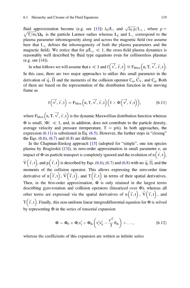
of them are based on the representation of the distribution function in the moving
frame as
f
v
0
!
, r
! , t
¼ F Mxw
n, T, v
0
!
, r
!
, t
1 þ Φ
v
0
!
, r
!
, t
,
ð6:11Þ
where F Mxw
n, T, v
0
!
, r
!
, t
is the dynamic Maxwellian distribution function whereas
Φ is small, jΦj ( 1, and, in addition, does not contribute to the particle density,
average velocity and pressure (temperature, T ¼ p/n). In both approaches, the
expression (6.11) is substituted in Eq. (6.5). However, the further steps in “closing”
the Eqs. (6.6), (6.7) and (6.8) are different.
In the Chapman-Enskog approach [15] (adopted for “simple”, one ion species
plasma by Braginskii [13]), in zero-order approximation in small parameter ε, an
impact of Φ on particle transport is completely ignored and the evolution of n r
!
, t
,
V
!
r
!
, t
, and p r
!
, t
is described by Eqs. (6.6), (6.7) and (6.8) with no q
!
, Π
$
, and the
moments of the collision operator. This allows expressing the zero-order time
derivative of n r
!
, t
, V
!
r
! , t
, and T r
!
, t
in terms of their spatial derivatives.
Then, in the first-order approximation, Φ is only retained in the largest terms
describing gyro-rotation and collision operators (linearized over Φ), whereas all
other terms are expressed via the spatial derivatives of n r
!
, t
, V
!
r
! , t
, and
T r
!
, t
. Finally, this non-uniform linear integrodifferential equation for Φ is solved
by representing Φ in the series of tensorial expansion
Φ ¼ Φ 0 þ Φ i v
0
i þ Φ ik v
0
i v
0
k À
v
0 2
3
δ ik
þ . . . ,
ð6:12Þ
whereas the coefficients of this expansion are written as infinite series
6.1 Hierarchy and Closure of the Fluid Equations
119
ffiffiffiffiffiffiffiffi
λ C ρ
p
=L ⊥ , where ρ ¼
ffiffiffiffiffiffiffiffiffi ffi
T=m
p
=Ω B is the particle Larmor radius whereas L k and L ⊥ correspond to the
plasma parameter inhomogeneity along and across the magnetic field (we assume
here that L ⊥ defines the inhomogeneity of both the plasma parameters and the
magnetic field). We notice that for ρ/L ⊥ ( 1, the cross-field plasma dynamics is
reasonably well described by fluid type equations even for collisionless plasmas
(e.g. see [14]).
In what follows we will assume that ε ( 1 and f
v
0
!
, r
! , t
ffi F Mxw
n, T, v
0
!
, r
! , t
.
In this case, there are two major approaches to utilize this small parameter in the
derivation of q
! , Π
$
and the moments of the collision operator C n , C
!
V , and C p . Both
of them are based on the representation of the distribution function in the moving
frame as
f
v
0
!
, r
! , t
¼ F Mxw
n, T, v
0
!
, r
!
, t
1 þ Φ
v
0
!
, r
!
, t
,
ð6:11Þ
where F Mxw
n, T, v
0
!
, r
!
, t
is the dynamic Maxwellian distribution function whereas
Φ is small, jΦj ( 1, and, in addition, does not contribute to the particle density,
average velocity and pressure (temperature, T ¼ p/n). In both approaches, the
expression (6.11) is substituted in Eq. (6.5). However, the further steps in “closing”
the Eqs. (6.6), (6.7) and (6.8) are different.
In the Chapman-Enskog approach [15] (adopted for “simple”, one ion species
plasma by Braginskii [13]), in zero-order approximation in small parameter ε, an
impact of Φ on particle transport is completely ignored and the evolution of n r
!
, t
,
V
!
r
!
, t
, and p r
!
, t
is described by Eqs. (6.6), (6.7) and (6.8) with no q
!
, Π
$
, and the
moments of the collision operator. This allows expressing the zero-order time
derivative of n r
!
, t
, V
!
r
! , t
, and T r
!
, t
in terms of their spatial derivatives.
Then, in the first-order approximation, Φ is only retained in the largest terms
describing gyro-rotation and collision operators (linearized over Φ), whereas all
other terms are expressed via the spatial derivatives of n r
!
, t
, V
!
r
! , t
, and
T r
!
, t
. Finally, this non-uniform linear integrodifferential equation for Φ is solved
by representing Φ in the series of tensorial expansion
Φ ¼ Φ 0 þ Φ i v
0
i þ Φ ik v
0
i v
0
k À
v
0 2
3
δ ik
þ . . . ,
ð6:12Þ
whereas the coefficients of this expansion are written as infinite series
6.1 Hierarchy and Closure of the Fluid Equations
119