

72
3 Analysis of Strain
∂
2 f
∂ y 2 =
∂
3 u
∂ x ∂ y 2
(3.34)
∂
2 g
∂ x 2 =
∂
3 v
∂ y ∂ x 2
(3.35)
∂
2 h
∂ x ∂ y
=
∂
3 v
∂ x 2 ∂ y
+
∂
3 u
∂ x ∂ y 2
(3.36)
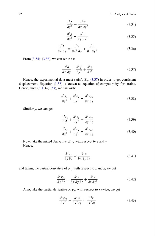
From (3.34)–(3.36), we can write as:
∂
2 h
∂ x ∂ y
=
∂
2 f
∂ y 2 +
∂
2 g
∂ x 2
(3.37)
Hence, the experimental data must satisfy Eq. (3.37) in order to get consistent
displacement. Equation (3.37) is known as equation of compatibility for strains.
Hence, from (3.31)–(3.33), we can write.
∂
2
ε x
∂ y 2 +
∂
2
ε y
∂ x 2 =
∂
2
γ xy
∂ x ∂ y
(3.38)
Similarly, we can get
∂
2
ε y
∂z 2 +
∂
2
ε z
∂ y 2 =
∂
2
γ yz
∂ y ∂z
(3.39)
∂
2
ε z
∂ x 2 +
∂
2
ε x
∂z 2 =
∂
2
γ zx
∂ x ∂z
(3.40)
Now, take the mixed derivative of ε x with respect to z and y,
Hence,
∂
2
ε x
∂ y ∂z
=
∂
3 u
∂ x ∂ y ∂z
(3.41)
and taking the partial derivative of γ xy with respect to z and x, we get
∂
2
γ xy
∂ x ∂z
=
∂
3 u
∂ x ∂ y ∂z
+
∂
3 v
∂z ∂ x 2
(3.42)
Also, take the partial derivative of γ yz with respect to x twice, we get
∂
2
γ yz
∂ x 2 =
∂
3 w
∂ x 2 ∂ y
+
∂
3 v
∂ x 2 ∂z
(3.43)
3 Analysis of Strain
∂
2 f
∂ y 2 =
∂
3 u
∂ x ∂ y 2
(3.34)
∂
2 g
∂ x 2 =
∂
3 v
∂ y ∂ x 2
(3.35)
∂
2 h
∂ x ∂ y
=
∂
3 v
∂ x 2 ∂ y
+
∂
3 u
∂ x ∂ y 2
(3.36)
From (3.34)–(3.36), we can write as:
∂
2 h
∂ x ∂ y
=
∂
2 f
∂ y 2 +
∂
2 g
∂ x 2
(3.37)
Hence, the experimental data must satisfy Eq. (3.37) in order to get consistent
displacement. Equation (3.37) is known as equation of compatibility for strains.
Hence, from (3.31)–(3.33), we can write.
∂
2
ε x
∂ y 2 +
∂
2
ε y
∂ x 2 =
∂
2
γ xy
∂ x ∂ y
(3.38)
Similarly, we can get
∂
2
ε y
∂z 2 +
∂
2
ε z
∂ y 2 =
∂
2
γ yz
∂ y ∂z
(3.39)
∂
2
ε z
∂ x 2 +
∂
2
ε x
∂z 2 =
∂
2
γ zx
∂ x ∂z
(3.40)
Now, take the mixed derivative of ε x with respect to z and y,
Hence,
∂
2
ε x
∂ y ∂z
=
∂
3 u
∂ x ∂ y ∂z
(3.41)
and taking the partial derivative of γ xy with respect to z and x, we get
∂
2
γ xy
∂ x ∂z
=
∂
3 u
∂ x ∂ y ∂z
+
∂
3 v
∂z ∂ x 2
(3.42)
Also, take the partial derivative of γ yz with respect to x twice, we get
∂
2
γ yz
∂ x 2 =
∂
3 w
∂ x 2 ∂ y
+
∂
3 v
∂ x 2 ∂z
(3.43)