

5.3 Transformation of Compatibility Equation from Strain Component …
131
(1 − ν)
∂
2
σ x
∂ y 2 +
∂
2
σ y
∂ x 2
− ν
∂
2
σ y
∂ y 2 +
∂
2
σ x
∂ x 2
= 2
∂
2
τ xy
∂ x ∂ y
(5.20)
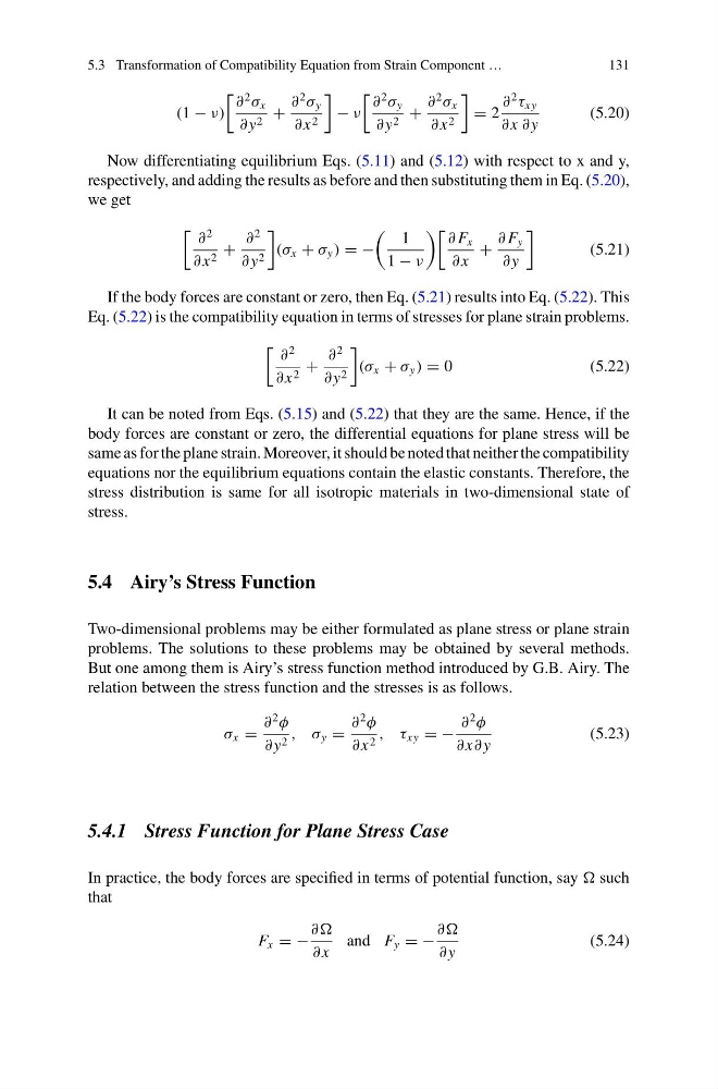
Now differentiating equilibrium Eqs. (5.11) and (5.12) with respect to x and y,
respectively, and adding the results as before and then substituting them in Eq. (5.20),
we get
∂
2
∂ x 2 +
∂
2
∂ y 2
(σ x + σ y ) = −
1
1 − ν
∂ F x
∂ x
+
∂ F y
∂ y
(5.21)
If the body forces are constant or zero, then Eq. (5.21) results into Eq. (5.22). This
Eq. (5.22) is the compatibility equation in terms of stresses for plane strain problems.
∂
2
∂ x 2 +
∂
2
∂ y 2
(σ x + σ y ) = 0
(5.22)
It can be noted from Eqs. (5.15) and (5.22) that they are the same. Hence, if the
body forces are constant or zero, the differential equations for plane stress will be
same as for the plane strain. Moreover, it should be noted that neither the compatibility
equations nor the equilibrium equations contain the elastic constants. Therefore, the
stress distribution is same for all isotropic materials in two-dimensional state of
stress.
5.4 Airy’s Stress Function
Two-dimensional problems may be either formulated as plane stress or plane strain
problems. The solutions to these problems may be obtained by several methods.
But one among them is Airy’s stress function method introduced by G.B. Airy. The
relation between the stress function and the stresses is as follows.
σ x =
∂
2
φ
∂ y 2 , σ y =
∂
2
φ
∂ x 2 , τ xy = −
∂
2
φ
∂ x∂ y
(5.23)
5.4.1 Stress Function for Plane Stress Case
In practice, the body forces are specified in terms of potential function, say such
that
F x = −
∂∂
∂ x
and F y = −
∂∂
∂ y
(5.24)
131
(1 − ν)
∂
2
σ x
∂ y 2 +
∂
2
σ y
∂ x 2
− ν
∂
2
σ y
∂ y 2 +
∂
2
σ x
∂ x 2
= 2
∂
2
τ xy
∂ x ∂ y
(5.20)
Now differentiating equilibrium Eqs. (5.11) and (5.12) with respect to x and y,
respectively, and adding the results as before and then substituting them in Eq. (5.20),
we get
∂
2
∂ x 2 +
∂
2
∂ y 2
(σ x + σ y ) = −
1
1 − ν
∂ F x
∂ x
+
∂ F y
∂ y
(5.21)
If the body forces are constant or zero, then Eq. (5.21) results into Eq. (5.22). This
Eq. (5.22) is the compatibility equation in terms of stresses for plane strain problems.
∂
2
∂ x 2 +
∂
2
∂ y 2
(σ x + σ y ) = 0
(5.22)
It can be noted from Eqs. (5.15) and (5.22) that they are the same. Hence, if the
body forces are constant or zero, the differential equations for plane stress will be
same as for the plane strain. Moreover, it should be noted that neither the compatibility
equations nor the equilibrium equations contain the elastic constants. Therefore, the
stress distribution is same for all isotropic materials in two-dimensional state of
stress.
5.4 Airy’s Stress Function
Two-dimensional problems may be either formulated as plane stress or plane strain
problems. The solutions to these problems may be obtained by several methods.
But one among them is Airy’s stress function method introduced by G.B. Airy. The
relation between the stress function and the stresses is as follows.
σ x =
∂
2
φ
∂ y 2 , σ y =
∂
2
φ
∂ x 2 , τ xy = −
∂
2
φ
∂ x∂ y
(5.23)
5.4.1 Stress Function for Plane Stress Case
In practice, the body forces are specified in terms of potential function, say such
that
F x = −
∂∂
∂ x
and F y = −
∂∂
∂ y
(5.24)