

4.8 Observer Space-Time
79
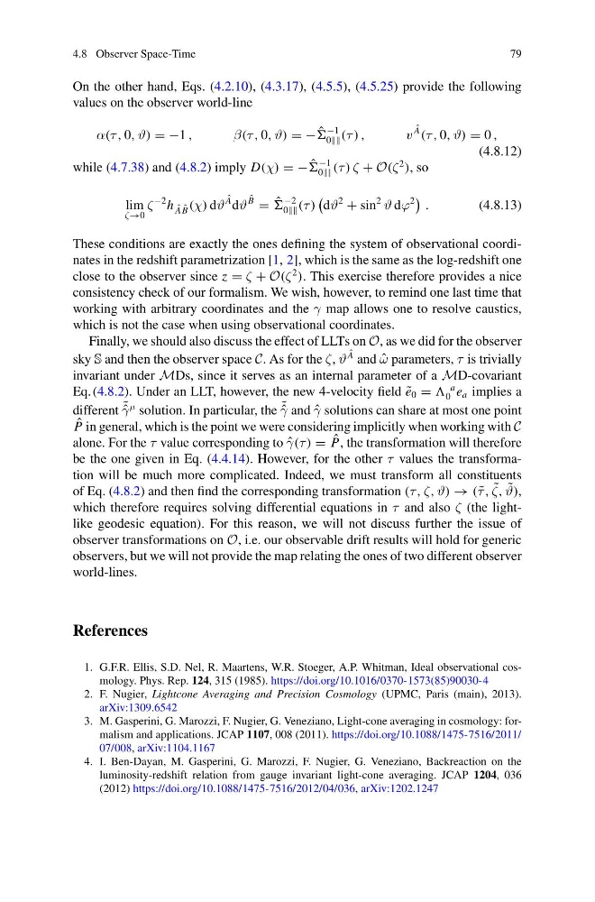
On the other hand, Eqs. (4.2.10), (4.3.17), (4.5.5), (4.5.25) provide the following
values on the observer world-line
α(τ , 0, ϑ) = −1 ,
β(τ , 0, ϑ) = − ˆ
−1
0 (τ ) ,
v
ˆ
A
(τ , 0, ϑ) = 0 ,
(4.8.12)
while (4.7.38) and (4.8.2) imply D(χ) = − ˆ
−1
0 (τ ) ζ + O(ζ
2
), so
lim
ζ→0
ζ
−2 h ˆ
A ˆ
B (χ) dϑ
ˆ
A dϑ
ˆ
B
= ˆ
−2
0 (τ )
dϑ
2
+ sin
2
ϑ dϕ
2
.
(4.8.13)
These conditions are exactly the ones defining the system of observational coordinates in the redshift parametrization [1, 2], which is the same as the log-redshift one
close to the observer since z = ζ + O(ζ
2
). This exercise therefore provides a nice
consistency check of our formalism. We wish, however, to remind one last time that
working with arbitrary coordinates and the γ map allows one to resolve caustics,
which is not the case when using observational coordinates.
Finally, we should also discuss the effect of LLTs on O, as we did for the observer
sky S and then the observer space C. As for the ζ, ϑ
ˆ
A and ˆ
ω parameters, τ is trivially
invariant under MDs, since it serves as an internal parameter of a MD-covariant
Eq. (4.8.2). Under an LLT, however, the new 4-velocity field ˜
e 0 =
a
0 e a implies a
different ˜ ˆ
γ
μ solution. In particular, the ˜ ˆ
γ and ˆ
γ solutions can share at most one point
ˆ
P in general, which is the point we were considering implicitly when working with C
alone. For the τ value corresponding to ˆ
γ(τ ) = ˆ
P, the transformation will therefore
be the one given in Eq. (4.4.14). However, for the other τ values the transformation will be much more complicated. Indeed, we must transform all constituents
of Eq. (4.8.2) and then find the corresponding transformation (τ , ζ, ϑ) → ( ˜
τ , ˜
ζ, ˜
ϑ),
which therefore requires solving differential equations in τ and also ζ (the lightlike geodesic equation). For this reason, we will not discuss further the issue of
observer transformations on O, i.e. our observable drift results will hold for generic
observers, but we will not provide the map relating the ones of two different observer
world-lines.
References
1. G.F.R. Ellis, S.D. Nel, R. Maartens, W.R. Stoeger, A.P. Whitman, Ideal observational cosmology. Phys. Rep. 124, 315 (1985). https://doi.org/10.1016/0370-1573(85)90030-4
2. F. Nugier, Lightcone Averaging and Precision Cosmology (UPMC, Paris (main), 2013).
arXiv:1309.6542
3. M. Gasperini, G. Marozzi, F. Nugier, G. Veneziano, Light-cone averaging in cosmology: formalism and applications. JCAP 1107, 008 (2011). https://doi.org/10.1088/1475-7516/2011/
07/008, arXiv:1104.1167
4. I. Ben-Dayan, M. Gasperini, G. Marozzi, F. Nugier, G. Veneziano, Backreaction on the
luminosity-redshift relation from gauge invariant light-cone averaging. JCAP 1204, 036
(2012) https://doi.org/10.1088/1475-7516/2012/04/036, arXiv:1202.1247
79
On the other hand, Eqs. (4.2.10), (4.3.17), (4.5.5), (4.5.25) provide the following
values on the observer world-line
α(τ , 0, ϑ) = −1 ,
β(τ , 0, ϑ) = − ˆ
−1
0 (τ ) ,
v
ˆ
A
(τ , 0, ϑ) = 0 ,
(4.8.12)
while (4.7.38) and (4.8.2) imply D(χ) = − ˆ
−1
0 (τ ) ζ + O(ζ
2
), so
lim
ζ→0
ζ
−2 h ˆ
A ˆ
B (χ) dϑ
ˆ
A dϑ
ˆ
B
= ˆ
−2
0 (τ )
dϑ
2
+ sin
2
ϑ dϕ
2
.
(4.8.13)
These conditions are exactly the ones defining the system of observational coordinates in the redshift parametrization [1, 2], which is the same as the log-redshift one
close to the observer since z = ζ + O(ζ
2
). This exercise therefore provides a nice
consistency check of our formalism. We wish, however, to remind one last time that
working with arbitrary coordinates and the γ map allows one to resolve caustics,
which is not the case when using observational coordinates.
Finally, we should also discuss the effect of LLTs on O, as we did for the observer
sky S and then the observer space C. As for the ζ, ϑ
ˆ
A and ˆ
ω parameters, τ is trivially
invariant under MDs, since it serves as an internal parameter of a MD-covariant
Eq. (4.8.2). Under an LLT, however, the new 4-velocity field ˜
e 0 =
a
0 e a implies a
different ˜ ˆ
γ
μ solution. In particular, the ˜ ˆ
γ and ˆ
γ solutions can share at most one point
ˆ
P in general, which is the point we were considering implicitly when working with C
alone. For the τ value corresponding to ˆ
γ(τ ) = ˆ
P, the transformation will therefore
be the one given in Eq. (4.4.14). However, for the other τ values the transformation will be much more complicated. Indeed, we must transform all constituents
of Eq. (4.8.2) and then find the corresponding transformation (τ , ζ, ϑ) → ( ˜
τ , ˜
ζ, ˜
ϑ),
which therefore requires solving differential equations in τ and also ζ (the lightlike geodesic equation). For this reason, we will not discuss further the issue of
observer transformations on O, i.e. our observable drift results will hold for generic
observers, but we will not provide the map relating the ones of two different observer
world-lines.
References
1. G.F.R. Ellis, S.D. Nel, R. Maartens, W.R. Stoeger, A.P. Whitman, Ideal observational cosmology. Phys. Rep. 124, 315 (1985). https://doi.org/10.1016/0370-1573(85)90030-4
2. F. Nugier, Lightcone Averaging and Precision Cosmology (UPMC, Paris (main), 2013).
arXiv:1309.6542
3. M. Gasperini, G. Marozzi, F. Nugier, G. Veneziano, Light-cone averaging in cosmology: formalism and applications. JCAP 1107, 008 (2011). https://doi.org/10.1088/1475-7516/2011/
07/008, arXiv:1104.1167
4. I. Ben-Dayan, M. Gasperini, G. Marozzi, F. Nugier, G. Veneziano, Backreaction on the
luminosity-redshift relation from gauge invariant light-cone averaging. JCAP 1204, 036
(2012) https://doi.org/10.1088/1475-7516/2012/04/036, arXiv:1202.1247