

78
4 Observer Space-Time Formalism
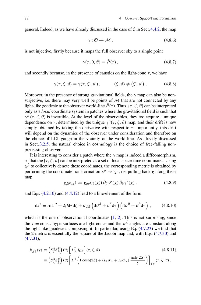
general. Indeed, as we have already discussed in the case of C in Sect. 4.4.2, the map
γ : O → M ,
(4.8.6)
is not injective, firstly because it maps the full observer sky to a single point
γ(τ , 0, ϑ) = ˆ
P(τ ) ,
(4.8.7)
and secondly because, in the presence of caustics on the light-cone τ , we have
γ(τ , ζ, ϑ) = γ(τ , ζ
, ϑ
) ,
(ζ, ϑ) =
ζ
, ϑ
.
(4.8.8)
Moreover, in the presence of strong gravitational fields, the γ map can also be nonsurjective, i.e. there may very well be points of M that are not connected by any
light-like geodesic to the observer world-line ˆ
P(τ ). Thus, {τ , ζ, ϑ} can be interpreted
only as a local coordinate system in patches where the gravitational field is such that
γ
μ
(τ , ζ, ϑ) is invertible. At the level of the observables, they too acquire a unique
dependence on τ , determined by the unique γ
μ
(τ , ζ, ϑ) map, and their drift is now
simply obtained by taking the derivative with respect to τ . Importantly, this drift
will depend on the dynamics of the observer under consideration and therefore on
the choice of LLT gauge in the vicinity of the world-line. As already discussed
in Sect. 3.2.5, the natural choice in cosmology is the choice of free-falling nonprecessing observers.
It is interesting to consider a patch where the γ map is indeed a diffeomorphism,
so that the {τ , ζ, ϑ} can be interpreted as a set of local space-time coordinates. Using
χ
ˆ
μ to collectively denote these coordinates, the corresponding metric is obtained by
performing the coordinate transformation x
μ
→ χ
ˆ
μ , i.e. pulling back g along the γ
map
g ˆ
μ ˆ
ν (χ) := g μν (γ(χ)) ∂ ˆ
μ γ
μ
(χ) ∂ ˆ
ν γ
ν
(χ) ,
(4.8.9)
and Eqs. (4.2.10) and (4.4.12) lead to a line-element of the form
ds
2
= αdτ
2
+ 2βdτ dζ + h ˆ
A ˆ
B
dϑ
ˆ
A
+ v
ˆ
A dτ
dϑ
ˆ
B
+ v
ˆ
B dτ
,
(4.8.10)
which is the one of observational coordinates [1, 2]. This is not surprising, since
the τ = const. hypersurfaces are light-cones and the ϑ
ˆ
A angles are constant along
the light-like geodesics composing it. In particular, using Eq. (4.7.23) we find that
the 2-metric is essentially the square of the Jacobi map and, with Eqs. (4.7.30) and
(4.7.31),
h ˆ
A ˆ
B (χ) ≡
S
A
ˆ
A
S
B
ˆ
B
(ϑ)
J
C
A J C B
(τ , ζ, ϑ)
(4.8.11)
≡
S
A
ˆ
A
S
B
ˆ
B
(ϑ)
D
2
1 cosh(2S) + (s + σ + + s × σ × )
sinh(2S)
S
AB
(τ , ζ, ϑ) .
4 Observer Space-Time Formalism
general. Indeed, as we have already discussed in the case of C in Sect. 4.4.2, the map
γ : O → M ,
(4.8.6)
is not injective, firstly because it maps the full observer sky to a single point
γ(τ , 0, ϑ) = ˆ
P(τ ) ,
(4.8.7)
and secondly because, in the presence of caustics on the light-cone τ , we have
γ(τ , ζ, ϑ) = γ(τ , ζ
, ϑ
) ,
(ζ, ϑ) =
ζ
, ϑ
.
(4.8.8)
Moreover, in the presence of strong gravitational fields, the γ map can also be nonsurjective, i.e. there may very well be points of M that are not connected by any
light-like geodesic to the observer world-line ˆ
P(τ ). Thus, {τ , ζ, ϑ} can be interpreted
only as a local coordinate system in patches where the gravitational field is such that
γ
μ
(τ , ζ, ϑ) is invertible. At the level of the observables, they too acquire a unique
dependence on τ , determined by the unique γ
μ
(τ , ζ, ϑ) map, and their drift is now
simply obtained by taking the derivative with respect to τ . Importantly, this drift
will depend on the dynamics of the observer under consideration and therefore on
the choice of LLT gauge in the vicinity of the world-line. As already discussed
in Sect. 3.2.5, the natural choice in cosmology is the choice of free-falling nonprecessing observers.
It is interesting to consider a patch where the γ map is indeed a diffeomorphism,
so that the {τ , ζ, ϑ} can be interpreted as a set of local space-time coordinates. Using
χ
ˆ
μ to collectively denote these coordinates, the corresponding metric is obtained by
performing the coordinate transformation x
μ
→ χ
ˆ
μ , i.e. pulling back g along the γ
map
g ˆ
μ ˆ
ν (χ) := g μν (γ(χ)) ∂ ˆ
μ γ
μ
(χ) ∂ ˆ
ν γ
ν
(χ) ,
(4.8.9)
and Eqs. (4.2.10) and (4.4.12) lead to a line-element of the form
ds
2
= αdτ
2
+ 2βdτ dζ + h ˆ
A ˆ
B
dϑ
ˆ
A
+ v
ˆ
A dτ
dϑ
ˆ
B
+ v
ˆ
B dτ
,
(4.8.10)
which is the one of observational coordinates [1, 2]. This is not surprising, since
the τ = const. hypersurfaces are light-cones and the ϑ
ˆ
A angles are constant along
the light-like geodesics composing it. In particular, using Eq. (4.7.23) we find that
the 2-metric is essentially the square of the Jacobi map and, with Eqs. (4.7.30) and
(4.7.31),
h ˆ
A ˆ
B (χ) ≡
S
A
ˆ
A
S
B
ˆ
B
(ϑ)
J
C
A J C B
(τ , ζ, ϑ)
(4.8.11)
≡
S
A
ˆ
A
S
B
ˆ
B
(ϑ)
D
2
1 cosh(2S) + (s + σ + + s × σ × )
sinh(2S)
S
AB
(τ , ζ, ϑ) .