

74
4 Observer Space-Time Formalism
∂ ζ D = −
1
e ζ 0
θ ,
(4.7.44)
∂ ζ s ◦ = −
1
e ζ D 0
1
S 2 (1 − S coth S) Re ( ¯
σs) s ◦ + Im ( ¯
σs)
,
(4.7.45)
∂ ζ s = −
1
e ζ D 0
(S coth S + is ◦ ) σ +
1
S 2 (1 − S coth S) Re ( ¯
σs) s
, (4.7.46)
∂ ζ θ =
1
0
1
e ζ D
|σ| 2 +
1
2
e ζ D R
,
(4.7.47)
∂ ζ σ =
1
0
1
e ζ D
θσ + e ζ D (W + + i W × )
.
(4.7.48)
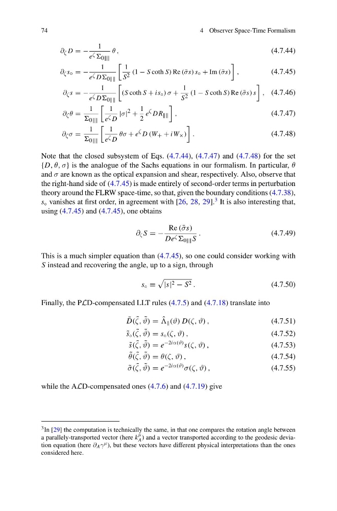
Note that the closed subsystem of Eqs. (4.7.44), (4.7.47) and (4.7.48) for the set
{D, θ, σ} is the analogue of the Sachs equations in our formalism. In particular, θ
and σ are known as the optical expansion and shear, respectively. Also, observe that
the right-hand side of (4.7.45) is made entirely of second-order terms in perturbation
theory around the FLRW space-time, so that, given the boundary conditions (4.7.38),
s ◦ vanishes at first order, in agreement with [26, 28, 29].
3 It is also interesting that,
using (4.7.45) and (4.7.45), one obtains
∂ ζ S = −
Re ( ¯
σs)
De ζ 0 S
.
(4.7.49)
This is a much simpler equation than (4.7.45), so one could consider working with
S instead and recovering the angle, up to a sign, through
s ◦ ≡
|s| 2 − S 2 .
(4.7.50)
Finally, the PLD-compensated LLT rules (4.7.5) and (4.7.18) translate into
˜
D( ˜
ζ, ˜
ϑ) = ˆ
(ϑ) D(ζ, ϑ) ,
(4.7.51)
˜
s ◦ ( ˜
ζ, ˜
ϑ) = s ◦ (ζ, ϑ) ,
(4.7.52)
˜
s( ˜
ζ, ˜
ϑ) = e
−2iα(ϑ) s(ζ, ϑ) ,
(4.7.53)
˜
θ( ˜
ζ, ˜
ϑ) = θ(ζ, ϑ) ,
(4.7.54)
˜
σ( ˜
ζ, ˜
ϑ) = e
−2iα(ϑ)
σ(ζ, ϑ) ,
(4.7.55)
while the ALD-compensated ones (4.7.6) and (4.7.19) give
3 In [29] the computation is technically the same, in that one compares the rotation angle between
a parallely-transported vector (here k
μ
A ) and a vector transported according to the geodesic deviation equation (here ∂ A γ μ ), but these vectors have different physical interpretations than the ones
considered here.
4 Observer Space-Time Formalism
∂ ζ D = −
1
e ζ 0
θ ,
(4.7.44)
∂ ζ s ◦ = −
1
e ζ D 0
1
S 2 (1 − S coth S) Re ( ¯
σs) s ◦ + Im ( ¯
σs)
,
(4.7.45)
∂ ζ s = −
1
e ζ D 0
(S coth S + is ◦ ) σ +
1
S 2 (1 − S coth S) Re ( ¯
σs) s
, (4.7.46)
∂ ζ θ =
1
0
1
e ζ D
|σ| 2 +
1
2
e ζ D R
,
(4.7.47)
∂ ζ σ =
1
0
1
e ζ D
θσ + e ζ D (W + + i W × )
.
(4.7.48)
Note that the closed subsystem of Eqs. (4.7.44), (4.7.47) and (4.7.48) for the set
{D, θ, σ} is the analogue of the Sachs equations in our formalism. In particular, θ
and σ are known as the optical expansion and shear, respectively. Also, observe that
the right-hand side of (4.7.45) is made entirely of second-order terms in perturbation
theory around the FLRW space-time, so that, given the boundary conditions (4.7.38),
s ◦ vanishes at first order, in agreement with [26, 28, 29].
3 It is also interesting that,
using (4.7.45) and (4.7.45), one obtains
∂ ζ S = −
Re ( ¯
σs)
De ζ 0 S
.
(4.7.49)
This is a much simpler equation than (4.7.45), so one could consider working with
S instead and recovering the angle, up to a sign, through
s ◦ ≡
|s| 2 − S 2 .
(4.7.50)
Finally, the PLD-compensated LLT rules (4.7.5) and (4.7.18) translate into
˜
D( ˜
ζ, ˜
ϑ) = ˆ
(ϑ) D(ζ, ϑ) ,
(4.7.51)
˜
s ◦ ( ˜
ζ, ˜
ϑ) = s ◦ (ζ, ϑ) ,
(4.7.52)
˜
s( ˜
ζ, ˜
ϑ) = e
−2iα(ϑ) s(ζ, ϑ) ,
(4.7.53)
˜
θ( ˜
ζ, ˜
ϑ) = θ(ζ, ϑ) ,
(4.7.54)
˜
σ( ˜
ζ, ˜
ϑ) = e
−2iα(ϑ)
σ(ζ, ϑ) ,
(4.7.55)
while the ALD-compensated ones (4.7.6) and (4.7.19) give
3 In [29] the computation is technically the same, in that one compares the rotation angle between
a parallely-transported vector (here k
μ
A ) and a vector transported according to the geodesic deviation equation (here ∂ A γ μ ), but these vectors have different physical interpretations than the ones
considered here.