

4.7 Observables from Localized Sources
73
From the first equation of (4.7.26) we then see that it is convenient to parametrize
K as
K = (θ1 + K c ) J c ,
K c := σ ◦ ε + σ + σ + + σ × σ × ,
σ := σ + + iσ × .
(4.7.37)
In terms of our new variables {D, s ◦ , s, θ, σ ◦ , σ}, the boundary conditions (4.7.7)
and (4.7.20) translate into
D(0, ϑ) = s ◦ (0, ϑ) = s(0, ϑ) = σ ◦ (0, ϑ) = σ(0, ϑ) = 0 ,
θ(0, ϑ) = 1 .
(4.7.38)
Let us now express (4.7.26) in terms of these variables. Multiplying the two equations
by J
−1
c from the right and splitting the result into pure-trace and traceless parts, we
obtain
∂ ζ D = −
θ
e ζ 0
,
Q c = −
1
e ζ D 0
K c ,
(4.7.39)
and
∂ ζ θ =
1
2 0
1
e ζ D
Tr (K
2
c ) + e
ζ D R
,
(4.7.40)
∂ ζ K c =
1
0
1
e ζ D
θ K c + e
ζ D (W + σ + + W × σ × )
,
(4.7.41)
where we have used the second equation of (4.7.39) to simplify the last two and
the fact that K
2
c ∼ 1. Before we proceed further, we note that the ∼ ε component of
(4.7.41), i.e. the evolution equation for σ ◦ , is a first-order linear differential equation
for σ ◦ with no source. Given the boundary condition (4.7.38) we therefore have
σ ◦ = 0 ,
(4.7.42)
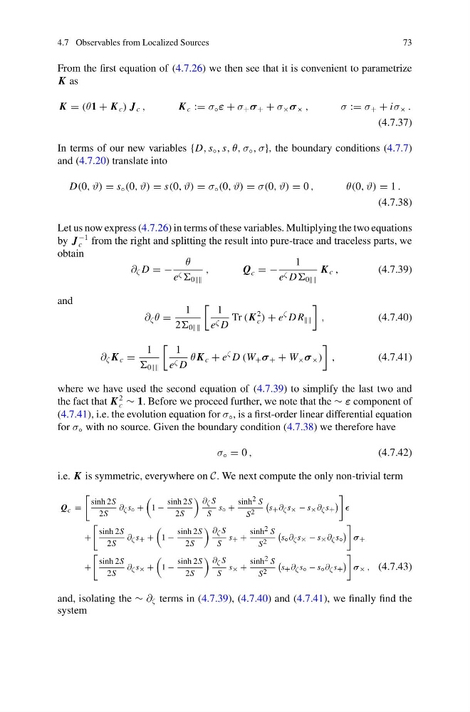
i.e. K is symmetric, everywhere on C. We next compute the only non-trivial term
Q c ≡
sinh 2S
2S
∂ ζ s ◦ +
1 −
sinh 2S
2S
∂ ζ S
S
s ◦ +
sinh 2 S
S 2
s + ∂ ζ s × − s × ∂ ζ s +
+
sinh 2S
2S
∂ ζ s + +
1 −
sinh 2S
2S
∂ ζ S
S
s + +
sinh 2 S
S 2
s ◦ ∂ ζ s × − s × ∂ ζ s ◦
σ +
+
sinh 2S
2S
∂ ζ s × +
1 −
sinh 2S
2S
∂ ζ S
S
s × +
sinh 2 S
S 2
s + ∂ ζ s ◦ − s ◦ ∂ ζ s +
σ × , (4.7.43)
and, isolating the ∼ ∂ ζ terms in (4.7.39), (4.7.40) and (4.7.41), we finally find the
system
73
From the first equation of (4.7.26) we then see that it is convenient to parametrize
K as
K = (θ1 + K c ) J c ,
K c := σ ◦ ε + σ + σ + + σ × σ × ,
σ := σ + + iσ × .
(4.7.37)
In terms of our new variables {D, s ◦ , s, θ, σ ◦ , σ}, the boundary conditions (4.7.7)
and (4.7.20) translate into
D(0, ϑ) = s ◦ (0, ϑ) = s(0, ϑ) = σ ◦ (0, ϑ) = σ(0, ϑ) = 0 ,
θ(0, ϑ) = 1 .
(4.7.38)
Let us now express (4.7.26) in terms of these variables. Multiplying the two equations
by J
−1
c from the right and splitting the result into pure-trace and traceless parts, we
obtain
∂ ζ D = −
θ
e ζ 0
,
Q c = −
1
e ζ D 0
K c ,
(4.7.39)
and
∂ ζ θ =
1
2 0
1
e ζ D
Tr (K
2
c ) + e
ζ D R
,
(4.7.40)
∂ ζ K c =
1
0
1
e ζ D
θ K c + e
ζ D (W + σ + + W × σ × )
,
(4.7.41)
where we have used the second equation of (4.7.39) to simplify the last two and
the fact that K
2
c ∼ 1. Before we proceed further, we note that the ∼ ε component of
(4.7.41), i.e. the evolution equation for σ ◦ , is a first-order linear differential equation
for σ ◦ with no source. Given the boundary condition (4.7.38) we therefore have
σ ◦ = 0 ,
(4.7.42)
i.e. K is symmetric, everywhere on C. We next compute the only non-trivial term
Q c ≡
sinh 2S
2S
∂ ζ s ◦ +
1 −
sinh 2S
2S
∂ ζ S
S
s ◦ +
sinh 2 S
S 2
s + ∂ ζ s × − s × ∂ ζ s +
+
sinh 2S
2S
∂ ζ s + +
1 −
sinh 2S
2S
∂ ζ S
S
s + +
sinh 2 S
S 2
s ◦ ∂ ζ s × − s × ∂ ζ s ◦
σ +
+
sinh 2S
2S
∂ ζ s × +
1 −
sinh 2S
2S
∂ ζ S
S
s × +
sinh 2 S
S 2
s + ∂ ζ s ◦ − s ◦ ∂ ζ s +
σ × , (4.7.43)
and, isolating the ∼ ∂ ζ terms in (4.7.39), (4.7.40) and (4.7.41), we finally find the
system