

4.7 Observables from Localized Sources
71
Also just like J AB , the transformation of K AB solely depends on LLTs at the observer
point ˆ
P. As for the boundary conditions, they are simply
ˆ
K AB (ϑ) := K AB (0, ϑ) = ˆ
n
i
A
ˆ
∂ B ˆ
n
i
≡ ˆ
n
i
A ˆ
n
i
B ≡ δ AB .
(4.7.20)
Using Eqs. (4.7.3), (4.7.12) and ∇ ζ k
a
= ∇ ζ k
a
A = 0, we then have that
∂ ζ J AB = −
K AB
e ζ 0
,
(4.7.21)
and
∂ ζ K AB = − ˆ
ω
−1 k
a
A ∇ ζ ∇ B k a = − ˆ
ω
−1 k
a
A
∇ ζ , ∇ B
k a =
e
ζ
0
R ab k
a
A e
b
μ ∂ B γ
μ
.
(4.7.22)
Now note that, because of (4.4.12), the combination e
a
μ ∂ A γ
μ obeys k a e
a
μ ∂ A γ
μ
= 0 and
therefore decomposes into a purely spatial part and a ∼ k
a part. From the definition
(4.7.3) of J AB we get
e
a
μ ∂ A γ
μ
=
0, n
i
B J
B
A
+ c A k
a
,
(4.7.23)
for some c A . Plugging this in (4.7.22), the antisymmetry of R abcd in its last two
indices eliminates the ∼ c A term and, using also (4.5.7), we finally get
∂ ζ K AB =
e
ζ
0
R AC J C B ,
(4.7.24)
where we have introduced the following notation for M-tensor fields evaluated on
γ
X n... := n
i X i... ,
X A... := n
i
A X i... .
(4.7.25)
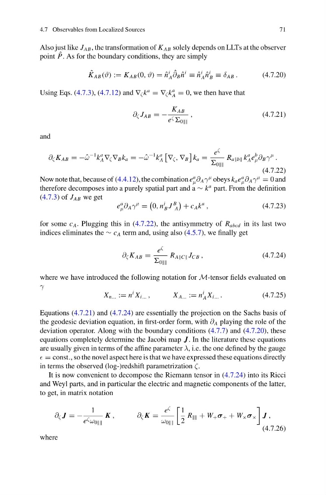
Equations (4.7.21) and (4.7.24) are essentially the projection on the Sachs basis of
the geodesic deviation equation, in first-order form, with ∂ A playing the role of the
deviation operator. Along with the boundary conditions (4.7.7) and (4.7.20), these
equations completely determine the Jacobi map J. In the literature these equations
are usually given in terms of the affine parameter λ, i.e. the one defined by the gauge
= const., so the novel aspect here is that we have expressed these equations directly
in terms the observed (log-)redshift parametrization ζ.
It is now convenient to decompose the Riemann tensor in (4.7.24) into its Ricci
and Weyl parts, and in particular the electric and magnetic components of the latter,
to get, in matrix notation
∂ ζ J = −
1
e ζ ω 0
K ,
∂ ζ K =
e
ζ
ω 0
1
2
R + W + σ + + W × σ ×
J ,
(4.7.26)
where
71
Also just like J AB , the transformation of K AB solely depends on LLTs at the observer
point ˆ
P. As for the boundary conditions, they are simply
ˆ
K AB (ϑ) := K AB (0, ϑ) = ˆ
n
i
A
ˆ
∂ B ˆ
n
i
≡ ˆ
n
i
A ˆ
n
i
B ≡ δ AB .
(4.7.20)
Using Eqs. (4.7.3), (4.7.12) and ∇ ζ k
a
= ∇ ζ k
a
A = 0, we then have that
∂ ζ J AB = −
K AB
e ζ 0
,
(4.7.21)
and
∂ ζ K AB = − ˆ
ω
−1 k
a
A ∇ ζ ∇ B k a = − ˆ
ω
−1 k
a
A
∇ ζ , ∇ B
k a =
e
ζ
0
R ab k
a
A e
b
μ ∂ B γ
μ
.
(4.7.22)
Now note that, because of (4.4.12), the combination e
a
μ ∂ A γ
μ obeys k a e
a
μ ∂ A γ
μ
= 0 and
therefore decomposes into a purely spatial part and a ∼ k
a part. From the definition
(4.7.3) of J AB we get
e
a
μ ∂ A γ
μ
=
0, n
i
B J
B
A
+ c A k
a
,
(4.7.23)
for some c A . Plugging this in (4.7.22), the antisymmetry of R abcd in its last two
indices eliminates the ∼ c A term and, using also (4.5.7), we finally get
∂ ζ K AB =
e
ζ
0
R AC J C B ,
(4.7.24)
where we have introduced the following notation for M-tensor fields evaluated on
γ
X n... := n
i X i... ,
X A... := n
i
A X i... .
(4.7.25)
Equations (4.7.21) and (4.7.24) are essentially the projection on the Sachs basis of
the geodesic deviation equation, in first-order form, with ∂ A playing the role of the
deviation operator. Along with the boundary conditions (4.7.7) and (4.7.20), these
equations completely determine the Jacobi map J. In the literature these equations
are usually given in terms of the affine parameter λ, i.e. the one defined by the gauge
= const., so the novel aspect here is that we have expressed these equations directly
in terms the observed (log-)redshift parametrization ζ.
It is now convenient to decompose the Riemann tensor in (4.7.24) into its Ricci
and Weyl parts, and in particular the electric and magnetic components of the latter,
to get, in matrix notation
∂ ζ J = −
1
e ζ ω 0
K ,
∂ ζ K =
e
ζ
ω 0
1
2
R + W + σ + + W × σ ×
J ,
(4.7.26)
where