

70
4 Observer Space-Time Formalism
d A :=
1
2
ε AB
n
A
i e
i
μ d ϑ γ
μ
∧
n
B
j e
j
ν d ϑ γ
ν
= [det J] d .
(4.7.10)
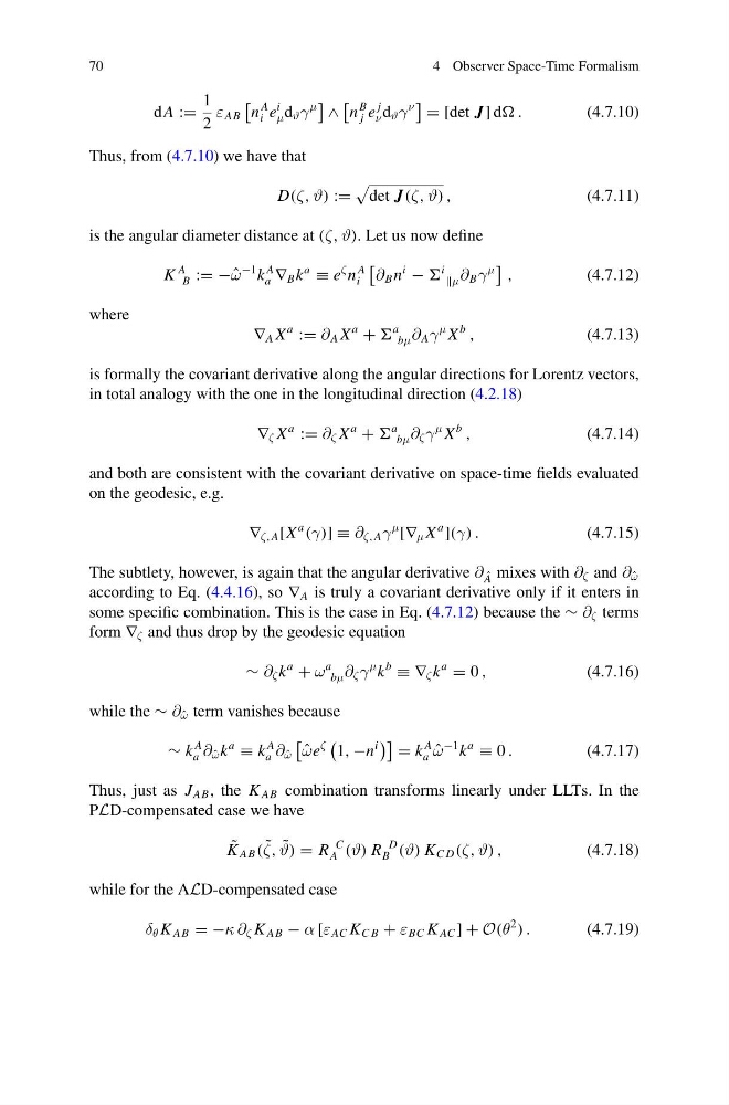
Thus, from (4.7.10) we have that
D(ζ, ϑ) :=
det J(ζ, ϑ) ,
(4.7.11)
is the angular diameter distance at (ζ, ϑ). Let us now define
K
A
B := − ˆ
ω
−1 k
A
a ∇ B k
a
≡ e
ζ n
A
i
∂ B n
i
−
i
μ ∂ B γ
μ
,
(4.7.12)
where
∇ A X
a
:= ∂ A X
a
+
a
bμ ∂ A γ
μ X
b
,
(4.7.13)
is formally the covariant derivative along the angular directions for Lorentz vectors,
in total analogy with the one in the longitudinal direction (4.2.18)
∇ ζ X
a
:= ∂ ζ X
a
+
a
bμ ∂ ζ γ
μ X
b
,
(4.7.14)
and both are consistent with the covariant derivative on space-time fields evaluated
on the geodesic, e.g.
∇ ζ,A [X
a
(γ)] ≡ ∂ ζ,A γ
μ
[∇ μ X
a
](γ) .
(4.7.15)
The subtlety, however, is again that the angular derivative ∂ ˆ
A mixes with ∂ ζ and ∂ ˆ
ω
according to Eq. (4.4.16), so ∇ A is truly a covariant derivative only if it enters in
some specific combination. This is the case in Eq. (4.7.12) because the ∼ ∂ ζ terms
form ∇ ζ and thus drop by the geodesic equation
∼ ∂ ζ k
a
+ ω
a
bμ ∂ ζ γ
μ k
b
≡ ∇ ζ k
a
= 0 ,
(4.7.16)
while the ∼ ∂ ˆ
ω term vanishes because
∼ k
A
a ∂ ˆ
ω k
a
≡ k
A
a ∂ ˆ
ω
ˆ
ωe
ζ
1, −n
i
= k
A
a ˆ
ω
−1 k
a
≡ 0 .
(4.7.17)
Thus, just as J AB , the K AB combination transforms linearly under LLTs. In the
PLD-compensated case we have
˜
K AB ( ˜
ζ, ˜
ϑ) = R
C
A (ϑ) R
D
B (ϑ) K C D (ζ, ϑ) ,
(4.7.18)
while for the ALD-compensated case
δ θ K AB = −κ ∂ ζ K AB − α [ε AC K C B + ε BC K AC ] + O(θ
2
) .
(4.7.19)
4 Observer Space-Time Formalism
d A :=
1
2
ε AB
n
A
i e
i
μ d ϑ γ
μ
∧
n
B
j e
j
ν d ϑ γ
ν
= [det J] d .
(4.7.10)
Thus, from (4.7.10) we have that
D(ζ, ϑ) :=
det J(ζ, ϑ) ,
(4.7.11)
is the angular diameter distance at (ζ, ϑ). Let us now define
K
A
B := − ˆ
ω
−1 k
A
a ∇ B k
a
≡ e
ζ n
A
i
∂ B n
i
−
i
μ ∂ B γ
μ
,
(4.7.12)
where
∇ A X
a
:= ∂ A X
a
+
a
bμ ∂ A γ
μ X
b
,
(4.7.13)
is formally the covariant derivative along the angular directions for Lorentz vectors,
in total analogy with the one in the longitudinal direction (4.2.18)
∇ ζ X
a
:= ∂ ζ X
a
+
a
bμ ∂ ζ γ
μ X
b
,
(4.7.14)
and both are consistent with the covariant derivative on space-time fields evaluated
on the geodesic, e.g.
∇ ζ,A [X
a
(γ)] ≡ ∂ ζ,A γ
μ
[∇ μ X
a
](γ) .
(4.7.15)
The subtlety, however, is again that the angular derivative ∂ ˆ
A mixes with ∂ ζ and ∂ ˆ
ω
according to Eq. (4.4.16), so ∇ A is truly a covariant derivative only if it enters in
some specific combination. This is the case in Eq. (4.7.12) because the ∼ ∂ ζ terms
form ∇ ζ and thus drop by the geodesic equation
∼ ∂ ζ k
a
+ ω
a
bμ ∂ ζ γ
μ k
b
≡ ∇ ζ k
a
= 0 ,
(4.7.16)
while the ∼ ∂ ˆ
ω term vanishes because
∼ k
A
a ∂ ˆ
ω k
a
≡ k
A
a ∂ ˆ
ω
ˆ
ωe
ζ
1, −n
i
= k
A
a ˆ
ω
−1 k
a
≡ 0 .
(4.7.17)
Thus, just as J AB , the K AB combination transforms linearly under LLTs. In the
PLD-compensated case we have
˜
K AB ( ˜
ζ, ˜
ϑ) = R
C
A (ϑ) R
D
B (ϑ) K C D (ζ, ϑ) ,
(4.7.18)
while for the ALD-compensated case
δ θ K AB = −κ ∂ ζ K AB − α [ε AC K C B + ε BC K AC ] + O(θ
2
) .
(4.7.19)