

6.2 Active and Passive Diffeomorphisms
135
˜
T
ν 1 ...ν n
μ 1 ...μ m
( ˜
x) =
∂ ˜
x
ν 1
∂ϕ σ 1
(ϕ( ˜
x)) . . .
∂ ˜
x
ν n
∂ϕ σ n
(ϕ( ˜
x))
∂ϕ
ρ 1
∂ ˜
x μ 1
( ˜
x) . . .
∂ϕ
ρ m
∂ ˜
x μ m
( ˜
x) T
σ 1 ...σ n
ρ 1 ...ρ m
(ϕ( ˜
x)) .
(6.2.6)
The reason we chose to express (6.2.6) in terms of ϕ
μ
( ˜
x), instead of x
μ
( ˜
x) as in
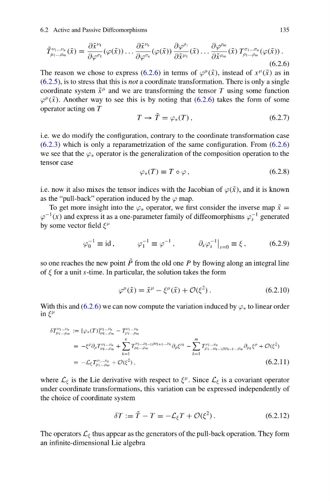
(6.2.5), is to stress that this is not a coordinate transformation. There is only a single
coordinate system ˜
x
μ and we are transforming the tensor T using some function
ϕ
μ
( ˜
x). Another way to see this is by noting that (6.2.6) takes the form of some
operator acting on T
T → ˜
T = ϕ ∗ (T ) ,
(6.2.7)
i.e. we do modify the configuration, contrary to the coordinate transformation case
(6.2.3) which is only a reparametrization of the same configuration. From (6.2.6)
we see that the ϕ ∗ operator is the generalization of the composition operation to the
tensor case
ϕ ∗ (T ) ≡ T ◦ ϕ ,
(6.2.8)
i.e. now it also mixes the tensor indices with the Jacobian of ϕ( ˜
x), and it is known
as the “pull-back” operation induced by the ϕ map.
To get more insight into the ϕ ∗ operator, we first consider the inverse map ˜
x =
ϕ
−1
(x) and express it as a one-parameter family of diffeomorphisms ϕ
−1
s generated
by some vector field ξ
μ
ϕ
−1
0 ≡ id ,
ϕ
−1
1 ≡ ϕ
−1
,
∂ s ϕ
−1
s
s=0
≡ ξ ,
(6.2.9)
so one reaches the new point ˜
P from the old one P by flowing along an integral line
of ξ for a unit s-time. In particular, the solution takes the form
ϕ
μ
( ˜
x) = ˜
x
μ
− ξ
μ
( ˜
x) + O(ξ
2
) .
(6.2.10)
With this and (6.2.6) we can now compute the variation induced by ϕ ∗ to linear order
in ξ
μ
δT
ν1...νn
μ1...μm := [ϕ ∗ (T )]
ν1...νn
μ1...μm − T
ν1...νn
μ1...μm
= −ξ
ρ ∂ ρ T
ν1...νn
μ1...μm +
n
k=1
T
ν1...νk−1ρνk+1...νn
μ1...μm
∂ ρ ξ
νk −
m
k=1
T
ν1...νn
μ1...μk−1ρμk+1...μm ∂ μk ξ
ρ + O(ξ
2 )
≡ −L ξ T
ν1...νn
μ1...μm + O(ξ
2 ) ,
(6.2.11)
where L ξ is the Lie derivative with respect to ξ
μ . Since L ξ is a covariant operator
under coordinate transformations, this variation can be expressed independently of
the choice of coordinate system
δT := ˜
T − T = −L ξ T + O(ξ
2
) .
(6.2.12)
The operators L ξ thus appear as the generators of the pull-back operation. They form
an infinite-dimensional Lie algebra
135
˜
T
ν 1 ...ν n
μ 1 ...μ m
( ˜
x) =
∂ ˜
x
ν 1
∂ϕ σ 1
(ϕ( ˜
x)) . . .
∂ ˜
x
ν n
∂ϕ σ n
(ϕ( ˜
x))
∂ϕ
ρ 1
∂ ˜
x μ 1
( ˜
x) . . .
∂ϕ
ρ m
∂ ˜
x μ m
( ˜
x) T
σ 1 ...σ n
ρ 1 ...ρ m
(ϕ( ˜
x)) .
(6.2.6)
The reason we chose to express (6.2.6) in terms of ϕ
μ
( ˜
x), instead of x
μ
( ˜
x) as in
(6.2.5), is to stress that this is not a coordinate transformation. There is only a single
coordinate system ˜
x
μ and we are transforming the tensor T using some function
ϕ
μ
( ˜
x). Another way to see this is by noting that (6.2.6) takes the form of some
operator acting on T
T → ˜
T = ϕ ∗ (T ) ,
(6.2.7)
i.e. we do modify the configuration, contrary to the coordinate transformation case
(6.2.3) which is only a reparametrization of the same configuration. From (6.2.6)
we see that the ϕ ∗ operator is the generalization of the composition operation to the
tensor case
ϕ ∗ (T ) ≡ T ◦ ϕ ,
(6.2.8)
i.e. now it also mixes the tensor indices with the Jacobian of ϕ( ˜
x), and it is known
as the “pull-back” operation induced by the ϕ map.
To get more insight into the ϕ ∗ operator, we first consider the inverse map ˜
x =
ϕ
−1
(x) and express it as a one-parameter family of diffeomorphisms ϕ
−1
s generated
by some vector field ξ
μ
ϕ
−1
0 ≡ id ,
ϕ
−1
1 ≡ ϕ
−1
,
∂ s ϕ
−1
s
s=0
≡ ξ ,
(6.2.9)
so one reaches the new point ˜
P from the old one P by flowing along an integral line
of ξ for a unit s-time. In particular, the solution takes the form
ϕ
μ
( ˜
x) = ˜
x
μ
− ξ
μ
( ˜
x) + O(ξ
2
) .
(6.2.10)
With this and (6.2.6) we can now compute the variation induced by ϕ ∗ to linear order
in ξ
μ
δT
ν1...νn
μ1...μm := [ϕ ∗ (T )]
ν1...νn
μ1...μm − T
ν1...νn
μ1...μm
= −ξ
ρ ∂ ρ T
ν1...νn
μ1...μm +
n
k=1
T
ν1...νk−1ρνk+1...νn
μ1...μm
∂ ρ ξ
νk −
m
k=1
T
ν1...νn
μ1...μk−1ρμk+1...μm ∂ μk ξ
ρ + O(ξ
2 )
≡ −L ξ T
ν1...νn
μ1...μm + O(ξ
2 ) ,
(6.2.11)
where L ξ is the Lie derivative with respect to ξ
μ . Since L ξ is a covariant operator
under coordinate transformations, this variation can be expressed independently of
the choice of coordinate system
δT := ˜
T − T = −L ξ T + O(ξ
2
) .
(6.2.12)
The operators L ξ thus appear as the generators of the pull-back operation. They form
an infinite-dimensional Lie algebra