

134
6 Appendix
and this leads to ˆ
g
tα
= 0. We thus have
ˆ
g
∂ μ , ∂ ν
≡ ˆ
g μν = η μν ,
ˆ
u = ˆ
∂ t ,
(6.1.6)
i.e. the ∂ μ basis is indeed orthonormal at ˆ
P.
6.2 Active and Passive Diffeomorphisms
The diffeomorphism symmetry of a differentiable manifold comes in two distinct
manifestations, differing both at the conceptual and practical levels. Here we consider
the space-time manifold M as our working example, but everything we discuss in
this section is applicable in general.
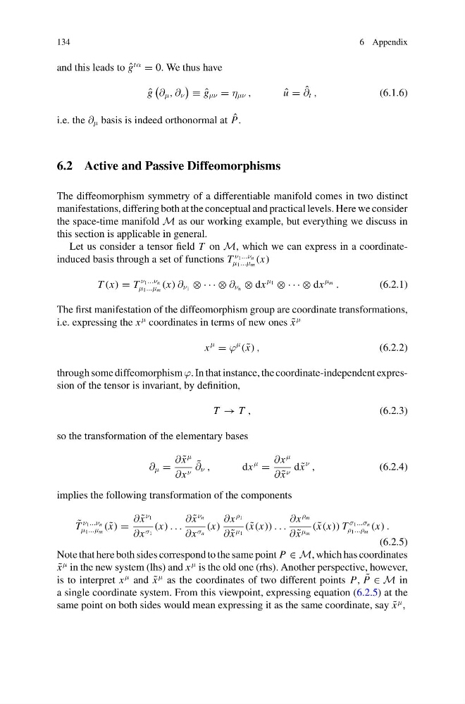
Let us consider a tensor field T on M, which we can express in a coordinateinduced basis through a set of functions T
ν 1 ...ν n
μ 1 ...μ m
(x)
T (x) = T
ν 1 ...ν n
μ 1 ...μ m
(x) ∂ ν 1 ⊗ · · · ⊗ ∂ ν n ⊗ dx
μ 1 ⊗ · · · ⊗ dx
μ m .
(6.2.1)
The first manifestation of the diffeomorphism group are coordinate transformations,
i.e. expressing the x
μ coordinates in terms of new ones ˜
x
μ
x
μ
= ϕ
μ
( ˜
x) ,
(6.2.2)
through some diffeomorphism ϕ. In that instance, the coordinate-independent expression of the tensor is invariant, by definition,
T → T ,
(6.2.3)
so the transformation of the elementary bases
∂ μ =
∂ ˜
x
μ
∂x ν
˜
∂ ν ,
dx
μ
=
∂x
μ
∂ ˜
x ν d ˜
x
ν
,
(6.2.4)
implies the following transformation of the components
˜
T
ν 1 ...ν n
μ 1 ...μ m
( ˜
x) =
∂ ˜
x
ν 1
∂x σ 1
(x) . . .
∂ ˜
x
ν n
∂x σ n
(x)
∂x
ρ 1
∂ ˜
x μ 1
( ˜
x(x)) . . .
∂x
ρ m
∂ ˜
x μ m
( ˜
x(x)) T
σ 1 ...σ n
ρ 1 ...ρ m
(x) .
(6.2.5)
Note that here both sides correspond to the same point P ∈ M, which has coordinates
˜
x
μ in the new system (lhs) and x
μ is the old one (rhs). Another perspective, however,
is to interpret x
μ and ˜
x
μ as the coordinates of two different points P, ˜
P ∈ M in
a single coordinate system. From this viewpoint, expressing equation (6.2.5) at the
same point on both sides would mean expressing it as the same coordinate, say ˜
x
μ ,
6 Appendix
and this leads to ˆ
g
tα
= 0. We thus have
ˆ
g
∂ μ , ∂ ν
≡ ˆ
g μν = η μν ,
ˆ
u = ˆ
∂ t ,
(6.1.6)
i.e. the ∂ μ basis is indeed orthonormal at ˆ
P.
6.2 Active and Passive Diffeomorphisms
The diffeomorphism symmetry of a differentiable manifold comes in two distinct
manifestations, differing both at the conceptual and practical levels. Here we consider
the space-time manifold M as our working example, but everything we discuss in
this section is applicable in general.
Let us consider a tensor field T on M, which we can express in a coordinateinduced basis through a set of functions T
ν 1 ...ν n
μ 1 ...μ m
(x)
T (x) = T
ν 1 ...ν n
μ 1 ...μ m
(x) ∂ ν 1 ⊗ · · · ⊗ ∂ ν n ⊗ dx
μ 1 ⊗ · · · ⊗ dx
μ m .
(6.2.1)
The first manifestation of the diffeomorphism group are coordinate transformations,
i.e. expressing the x
μ coordinates in terms of new ones ˜
x
μ
x
μ
= ϕ
μ
( ˜
x) ,
(6.2.2)
through some diffeomorphism ϕ. In that instance, the coordinate-independent expression of the tensor is invariant, by definition,
T → T ,
(6.2.3)
so the transformation of the elementary bases
∂ μ =
∂ ˜
x
μ
∂x ν
˜
∂ ν ,
dx
μ
=
∂x
μ
∂ ˜
x ν d ˜
x
ν
,
(6.2.4)
implies the following transformation of the components
˜
T
ν 1 ...ν n
μ 1 ...μ m
( ˜
x) =
∂ ˜
x
ν 1
∂x σ 1
(x) . . .
∂ ˜
x
ν n
∂x σ n
(x)
∂x
ρ 1
∂ ˜
x μ 1
( ˜
x(x)) . . .
∂x
ρ m
∂ ˜
x μ m
( ˜
x(x)) T
σ 1 ...σ n
ρ 1 ...ρ m
(x) .
(6.2.5)
Note that here both sides correspond to the same point P ∈ M, which has coordinates
˜
x
μ in the new system (lhs) and x
μ is the old one (rhs). Another perspective, however,
is to interpret x
μ and ˜
x
μ as the coordinates of two different points P, ˜
P ∈ M in
a single coordinate system. From this viewpoint, expressing equation (6.2.5) at the
same point on both sides would mean expressing it as the same coordinate, say ˜
x
μ ,