

5.8 Liouville-Transported Wave-Functions and Tensor Distributions
113
which obeys (5.8.20) as well. Finally, the inverse relation reads
I ≡ f
a
a ,
P ab ≡ 2 f (ab) − ab f
c
c ,
V ≡ −iε
ab f ab ,
(5.8.22)
and the BUU equation (5.8.8) turns into
LI = C
a
a ,
LV = −iε
ab C ab ,
L P ab = 2C (ab) − ab C
c
c . (5.8.23)
5.8.2 Dirac Fermions
We now consider the case of a Dirac particle of mass m and charge q, along with
its anti-particle. These correspond to two 2 × 2 blocks in f , which we denote
by f
±
ss (x,
p), s ∈ {1, 2}, with ± distinguishing the particle and anti-particle ones,
respectively. The on-shell 4-momentum therefore obeys p a p
a
≡ −m
2 and we will
focus exclusively on the massive case m = 0 for simplicity.
8
The wave-functions are the four Dirac spinor distributions {u
±
s (x,
p)} s=1,2 obeying the standard orthonormality relation
¯
u
±
s u
±
s ≡ ± 2mδ ss ,
¯
u
±
s u
∓
s ≡ 0 ,
¯
u := u
†
γ
0
,
(5.8.24)
the completeness relation
u
±
s (
p) ¯
u
±
s (
p) ≡ p ± m ,
(5.8.25)
and the Dirac equation
( p ∓ m) u
±
s (
p) ≡ 0 ,
p := γ
a p a ,
(5.8.26)
and relating the quantum field to the ladder operators as follows
ψ(X ) =
s=1,2
d
3 p
(2π) 3
2E p
u
+
s (
p) a
+
p,s e
i p a X
a + u
−
s (
p) (a
−
p,s )
† e
−i p a X
a
.
(5.8.27)
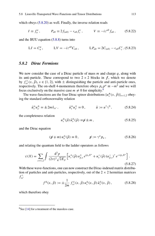
With these wave-functions, one can now construct the Dirac-indexed matrix distribution of particles and anti-particles, respectively, out of the 2 × 2 hermitian matrices
f
±
ss
f
±
(x,
p) := ±
1
2m
f
±
ss (x,
p) u
±
s (x,
p) ¯
u
±
s (x,
p) ,
(5.8.28)
which therefore obey
8 See [14] for a treatment of the massless case.
113
which obeys (5.8.20) as well. Finally, the inverse relation reads
I ≡ f
a
a ,
P ab ≡ 2 f (ab) − ab f
c
c ,
V ≡ −iε
ab f ab ,
(5.8.22)
and the BUU equation (5.8.8) turns into
LI = C
a
a ,
LV = −iε
ab C ab ,
L P ab = 2C (ab) − ab C
c
c . (5.8.23)
5.8.2 Dirac Fermions
We now consider the case of a Dirac particle of mass m and charge q, along with
its anti-particle. These correspond to two 2 × 2 blocks in f , which we denote
by f
±
ss (x,
p), s ∈ {1, 2}, with ± distinguishing the particle and anti-particle ones,
respectively. The on-shell 4-momentum therefore obeys p a p
a
≡ −m
2 and we will
focus exclusively on the massive case m = 0 for simplicity.
8
The wave-functions are the four Dirac spinor distributions {u
±
s (x,
p)} s=1,2 obeying the standard orthonormality relation
¯
u
±
s u
±
s ≡ ± 2mδ ss ,
¯
u
±
s u
∓
s ≡ 0 ,
¯
u := u
†
γ
0
,
(5.8.24)
the completeness relation
u
±
s (
p) ¯
u
±
s (
p) ≡ p ± m ,
(5.8.25)
and the Dirac equation
( p ∓ m) u
±
s (
p) ≡ 0 ,
p := γ
a p a ,
(5.8.26)
and relating the quantum field to the ladder operators as follows
ψ(X ) =
s=1,2
d
3 p
(2π) 3
2E p
u
+
s (
p) a
+
p,s e
i p a X
a + u
−
s (
p) (a
−
p,s )
† e
−i p a X
a
.
(5.8.27)
With these wave-functions, one can now construct the Dirac-indexed matrix distribution of particles and anti-particles, respectively, out of the 2 × 2 hermitian matrices
f
±
ss
f
±
(x,
p) := ±
1
2m
f
±
ss (x,
p) u
±
s (x,
p) ¯
u
±
s (x,
p) ,
(5.8.28)
which therefore obey
8 See [14] for a treatment of the massless case.