

110
5 General-Relativistic Matrix Kinetic Theory
scattering matrix elements that depend solely on the momenta, not depend on x
μ .
Here we will discuss the two examples cited above, since these are the most relevant
ones for cosmology.
5.8.1 Photons
We focus on the 2 × 2 block of f corresponding to the photon distribution. For
later convenience, and in order to remain close to the usual conventions, we will use
r to denote the indices of this matrix and k
a to denote the null 4-momentum, e.g.
f rr (x,
k). In this case the wave-functions are usually referred to as “polarization
vectors”
a
r (x,
k), r ∈ {1, 2}, which can be chosen such that
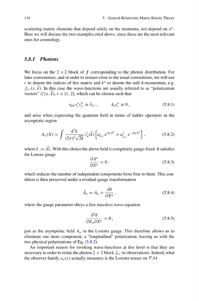
η ab
a
r
b
r ≡ δ rr ,
k a
a
r ≡ 0 ,
(5.8.1)
and arise when expressing the quantum field in terms of ladder operators in the
asymptotic region
A a (X ) =
d
3 k
(2π) 3
√
2k
r
a (
k)
a
k,r e
ik b X
b + a
†
k,r
e
−ik b X
b
,
(5.8.2)
where k := |
k|. With this choice the above field is completely gauge-fixed. It satisfies
the Lorenz gauge
∂ A
a
∂ X a = 0 ,
(5.8.3)
which reduces the number of independent components from four to three. This condition is then preserved under a residual gauge transformation
˜
A a = A a +
∂θ
∂ X a ,
(5.8.4)
where the gauge parameter obeys a free massless wave-equation
∂
2
θ
∂ X a ∂ X a = 0 ,
(5.8.5)
just as the asymptotic field A a in the Lorentz gauge. This therefore allows us to
eliminate one more component, a “longitudinal” polarization, leaving us with the
two physical polarizations of Eq. (5.8.2).
An important reason for invoking wave-functions at this level is that they are
necessary in order to relate the photon 2 × 2 block f rr to observations. Indeed, what
the observer family e a (x) actually measures is the Lorentz tensor on PM
5 General-Relativistic Matrix Kinetic Theory
scattering matrix elements that depend solely on the momenta, not depend on x
μ .
Here we will discuss the two examples cited above, since these are the most relevant
ones for cosmology.
5.8.1 Photons
We focus on the 2 × 2 block of f corresponding to the photon distribution. For
later convenience, and in order to remain close to the usual conventions, we will use
r to denote the indices of this matrix and k
a to denote the null 4-momentum, e.g.
f rr (x,
k). In this case the wave-functions are usually referred to as “polarization
vectors”
a
r (x,
k), r ∈ {1, 2}, which can be chosen such that
η ab
a
r
b
r ≡ δ rr ,
k a
a
r ≡ 0 ,
(5.8.1)
and arise when expressing the quantum field in terms of ladder operators in the
asymptotic region
A a (X ) =
d
3 k
(2π) 3
√
2k
r
a (
k)
a
k,r e
ik b X
b + a
†
k,r
e
−ik b X
b
,
(5.8.2)
where k := |
k|. With this choice the above field is completely gauge-fixed. It satisfies
the Lorenz gauge
∂ A
a
∂ X a = 0 ,
(5.8.3)
which reduces the number of independent components from four to three. This condition is then preserved under a residual gauge transformation
˜
A a = A a +
∂θ
∂ X a ,
(5.8.4)
where the gauge parameter obeys a free massless wave-equation
∂
2
θ
∂ X a ∂ X a = 0 ,
(5.8.5)
just as the asymptotic field A a in the Lorentz gauge. This therefore allows us to
eliminate one more component, a “longitudinal” polarization, leaving us with the
two physical polarizations of Eq. (5.8.2).
An important reason for invoking wave-functions at this level is that they are
necessary in order to relate the photon 2 × 2 block f rr to observations. Indeed, what
the observer family e a (x) actually measures is the Lorentz tensor on PM