

106
5 General-Relativistic Matrix Kinetic Theory
C 1↔n
ss (x,
p) =
1
2
⎛
⎝
n
k=1
d 3 p k
(2π) 3 2E p k ,s k
⎞
⎠ (2π) 4 δ (4)
⎛
⎝ p −
n
k=1
p k
⎞
⎠
×
f s 1 s
1
(x,
p 1 ) . . . f s n s
n
(x,
p n ) f ◦
s s (x,
p)
(5.5.23)
× A c (
p 1 , s 1 , . . . ,
p n , s n → →
p, s) A ∗
c (
p 1 , s
1 , . . . ,
p n , s
n → →
p, s )
− f ss (x,
p) f ◦
s
1 s 1
(x,
p 1 ) . . . f ◦
s
n s n
(x,
p n )
× A c (
p, s → →
p 1 , s 1 , . . . ,
p n , s n ) A ∗
c (
p, s → →
p 1 , s
1 , . . . ,
p n , s
n )
.
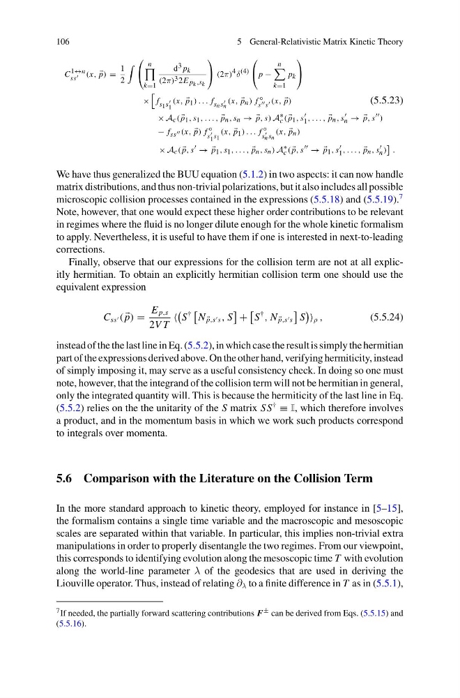
We have thus generalized the BUU equation (5.1.2) in two aspects: it can now handle
matrix distributions, and thus non-trivial polarizations, but it also includes all possible
microscopic collision processes contained in the expressions (5.5.18) and (5.5.19).
7
Note, however, that one would expect these higher order contributions to be relevant
in regimes where the fluid is no longer dilute enough for the whole kinetic formalism
to apply. Nevertheless, it is useful to have them if one is interested in next-to-leading
corrections.
Finally, observe that our expressions for the collision term are not at all explicitly hermitian. To obtain an explicitly hermitian collision term one should use the
equivalent expression
C ss (
p) =
E p,s
2V T
S
†
N
p,s s , S
+
S
†
, N
p,s s
S
ρ ,
(5.5.24)
instead of the the last line in Eq. (5.5.2), in which case the result is simply the hermitian
part of the expressions derived above. On the other hand, verifying hermiticity, instead
of simply imposing it, may serve as a useful consistency check. In doing so one must
note, however, that the integrand of the collision term will not be hermitian in general,
only the integrated quantity will. This is because the hermiticity of the last line in Eq.
(5.5.2) relies on the the unitarity of the S matrix SS
†
≡ I, which therefore involves
a product, and in the momentum basis in which we work such products correspond
to integrals over momenta.
5.6 Comparison with the Literature on the Collision Term
In the more standard approach to kinetic theory, employed for instance in [5–15],
the formalism contains a single time variable and the macroscopic and mesoscopic
scales are separated within that variable. In particular, this implies non-trivial extra
manipulations in order to properly disentangle the two regimes. From our viewpoint,
this corresponds to identifying evolution along the mesoscopic time T with evolution
along the world-line parameter λ of the geodesics that are used in deriving the
Liouville operator. Thus, instead of relating ∂ λ to a finite difference in T as in (5.5.1),
7 If needed, the partially forward scattering contributions F ± can be derived from Eqs. (5.5.15) and
(5.5.16).
5 General-Relativistic Matrix Kinetic Theory
C 1↔n
ss (x,
p) =
1
2
⎛
⎝
n
k=1
d 3 p k
(2π) 3 2E p k ,s k
⎞
⎠ (2π) 4 δ (4)
⎛
⎝ p −
n
k=1
p k
⎞
⎠
×
f s 1 s
1
(x,
p 1 ) . . . f s n s
n
(x,
p n ) f ◦
s s (x,
p)
(5.5.23)
× A c (
p 1 , s 1 , . . . ,
p n , s n → →
p, s) A ∗
c (
p 1 , s
1 , . . . ,
p n , s
n → →
p, s )
− f ss (x,
p) f ◦
s
1 s 1
(x,
p 1 ) . . . f ◦
s
n s n
(x,
p n )
× A c (
p, s → →
p 1 , s 1 , . . . ,
p n , s n ) A ∗
c (
p, s → →
p 1 , s
1 , . . . ,
p n , s
n )
.
We have thus generalized the BUU equation (5.1.2) in two aspects: it can now handle
matrix distributions, and thus non-trivial polarizations, but it also includes all possible
microscopic collision processes contained in the expressions (5.5.18) and (5.5.19).
7
Note, however, that one would expect these higher order contributions to be relevant
in regimes where the fluid is no longer dilute enough for the whole kinetic formalism
to apply. Nevertheless, it is useful to have them if one is interested in next-to-leading
corrections.
Finally, observe that our expressions for the collision term are not at all explicitly hermitian. To obtain an explicitly hermitian collision term one should use the
equivalent expression
C ss (
p) =
E p,s
2V T
S
†
N
p,s s , S
+
S
†
, N
p,s s
S
ρ ,
(5.5.24)
instead of the the last line in Eq. (5.5.2), in which case the result is simply the hermitian
part of the expressions derived above. On the other hand, verifying hermiticity, instead
of simply imposing it, may serve as a useful consistency check. In doing so one must
note, however, that the integrand of the collision term will not be hermitian in general,
only the integrated quantity will. This is because the hermiticity of the last line in Eq.
(5.5.2) relies on the the unitarity of the S matrix SS
†
≡ I, which therefore involves
a product, and in the momentum basis in which we work such products correspond
to integrals over momenta.
5.6 Comparison with the Literature on the Collision Term
In the more standard approach to kinetic theory, employed for instance in [5–15],
the formalism contains a single time variable and the macroscopic and mesoscopic
scales are separated within that variable. In particular, this implies non-trivial extra
manipulations in order to properly disentangle the two regimes. From our viewpoint,
this corresponds to identifying evolution along the mesoscopic time T with evolution
along the world-line parameter λ of the geodesics that are used in deriving the
Liouville operator. Thus, instead of relating ∂ λ to a finite difference in T as in (5.5.1),
7 If needed, the partially forward scattering contributions F ± can be derived from Eqs. (5.5.15) and
(5.5.16).