

11.6 Particle Image Velocimetry
253
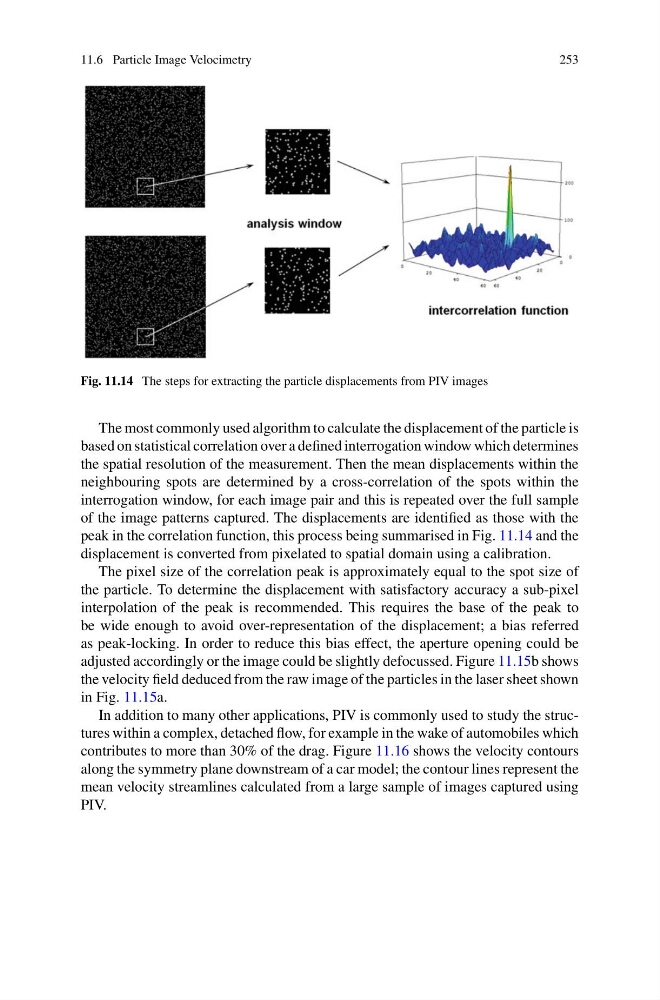
Fig. 11.14 The steps for extracting the particle displacements from PIV images
The most commonly used algorithm to calculate the displacement of the particle is
based on statistical correlation over a defined interrogation window which determines
the spatial resolution of the measurement. Then the mean displacements within the
neighbouring spots are determined by a cross-correlation of the spots within the
interrogation window, for each image pair and this is repeated over the full sample
of the image patterns captured. The displacements are identified as those with the
peak in the correlation function, this process being summarised in Fig. 11.14 and the
displacement is converted from pixelated to spatial domain using a calibration.
The pixel size of the correlation peak is approximately equal to the spot size of
the particle. To determine the displacement with satisfactory accuracy a sub-pixel
interpolation of the peak is recommended. This requires the base of the peak to
be wide enough to avoid over-representation of the displacement; a bias referred
as peak-locking. In order to reduce this bias effect, the aperture opening could be
adjusted accordingly or the image could be slightly defocussed. Figure 11.15b shows
the velocity field deduced from the raw image of the particles in the laser sheet shown
in Fig. 11.15a.
In addition to many other applications, PIV is commonly used to study the structures within a complex, detached flow, for example in the wake of automobiles which
contributes to more than 30% of the drag. Figure 11.16 shows the velocity contours
along the symmetry plane downstream of a car model; the contour lines represent the
mean velocity streamlines calculated from a large sample of images captured using
PIV.
253
Fig. 11.14 The steps for extracting the particle displacements from PIV images
The most commonly used algorithm to calculate the displacement of the particle is
based on statistical correlation over a defined interrogation window which determines
the spatial resolution of the measurement. Then the mean displacements within the
neighbouring spots are determined by a cross-correlation of the spots within the
interrogation window, for each image pair and this is repeated over the full sample
of the image patterns captured. The displacements are identified as those with the
peak in the correlation function, this process being summarised in Fig. 11.14 and the
displacement is converted from pixelated to spatial domain using a calibration.
The pixel size of the correlation peak is approximately equal to the spot size of
the particle. To determine the displacement with satisfactory accuracy a sub-pixel
interpolation of the peak is recommended. This requires the base of the peak to
be wide enough to avoid over-representation of the displacement; a bias referred
as peak-locking. In order to reduce this bias effect, the aperture opening could be
adjusted accordingly or the image could be slightly defocussed. Figure 11.15b shows
the velocity field deduced from the raw image of the particles in the laser sheet shown
in Fig. 11.15a.
In addition to many other applications, PIV is commonly used to study the structures within a complex, detached flow, for example in the wake of automobiles which
contributes to more than 30% of the drag. Figure 11.16 shows the velocity contours
along the symmetry plane downstream of a car model; the contour lines represent the
mean velocity streamlines calculated from a large sample of images captured using
PIV.