

11.2 Interferometry
239
= b
By choosing a reference fringe, the change in the optical path between two points,
R, and M, in the flow field can be expressed as a function of the fringe spacing:
= λ(N M − N R ) = b(n M − n R )
where λ is the wavelength of the light source, and N R and N M the fringe numbers
between points R and M respectively. If the flow is two-dimensional, the density, ρ
does not vary along the spanwise direction. Assuming that, b = l, the value of ρ at
a point N M within the fringe is expressed by the following relation:
ρ M = ρ R +
λ
bB
(N M − N R )
where ρ R is the value of ρ corresponding to the reference fringe N R . This value is
determined by considering a fringe passing in a region of uniform flow where the
temperature and pressure can be measured.
In practice each fringe, black or white, is identified by its median line where
the light intensity changes from maximum to minimum or the two extremes of the
grey scale intensity (in theory it should be possible to divide the main fringe into
multiple fractions of fringes but this is not very accurate). The main issue with the
interferogram is to identify the centre of each fringe; however this could be resolved
more accurately nowadays using more advanced image processing routine. Once the
centre of each fringe has been identified, the density field, ρ(x, y) over a 2D plane
can be determined within the experimental domain.
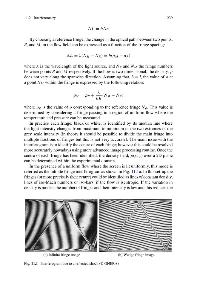
In the presence of a uniform flow where the screen is lit uniformly, this mode is
referred as the infinite fringe interferogram as shown in Fig. 11.1a. In this set-up the
fringes (or more precisely their centre) could be identified as lines of constant density,
lines of iso-Mach numbers or iso-bars, if the flow is isentropic. If the variation in
density is modest the number of fringes and their intensity is low and this reduces the
(a) Infinite fringe image
(b) Wedge fringe image
Fig. 11.1 Interferogram due to a reflected shock (© ONERA)
239
= b
By choosing a reference fringe, the change in the optical path between two points,
R, and M, in the flow field can be expressed as a function of the fringe spacing:
= λ(N M − N R ) = b(n M − n R )
where λ is the wavelength of the light source, and N R and N M the fringe numbers
between points R and M respectively. If the flow is two-dimensional, the density, ρ
does not vary along the spanwise direction. Assuming that, b = l, the value of ρ at
a point N M within the fringe is expressed by the following relation:
ρ M = ρ R +
λ
bB
(N M − N R )
where ρ R is the value of ρ corresponding to the reference fringe N R . This value is
determined by considering a fringe passing in a region of uniform flow where the
temperature and pressure can be measured.
In practice each fringe, black or white, is identified by its median line where
the light intensity changes from maximum to minimum or the two extremes of the
grey scale intensity (in theory it should be possible to divide the main fringe into
multiple fractions of fringes but this is not very accurate). The main issue with the
interferogram is to identify the centre of each fringe; however this could be resolved
more accurately nowadays using more advanced image processing routine. Once the
centre of each fringe has been identified, the density field, ρ(x, y) over a 2D plane
can be determined within the experimental domain.
In the presence of a uniform flow where the screen is lit uniformly, this mode is
referred as the infinite fringe interferogram as shown in Fig. 11.1a. In this set-up the
fringes (or more precisely their centre) could be identified as lines of constant density,
lines of iso-Mach numbers or iso-bars, if the flow is isentropic. If the variation in
density is modest the number of fringes and their intensity is low and this reduces the
(a) Infinite fringe image
(b) Wedge fringe image
Fig. 11.1 Interferogram due to a reflected shock (© ONERA)