

4 Light-Dressed Spectroscopy of Molecules
85
(F)
I | I (t) =
l,k
a
∗
l b k e
−
i
(εk −εl )t0 l (t 0 )| k (t 0 )
+
1
i
l,k
a
∗
l b k
t
t0
e
−
i
(εk −εl )t0 l (t 0 )| ˆ
W 2I (t
)| k (t 0 )dt
=
l,k
a
∗
l b k e
−
i
(εk −εl )t0 l (t 0 )| k (t 0 )
+
1
i
l,k
a
∗
l b k
t
t0
e
−
i
(εk −εl )t0 l (t 0 )|e
i
t
t 0
ˆ
Hd (t )dt
ˆ
W 2 (t
)e
−
i
t
t 0
ˆ
Hd (t )dt
| k (t 0 )dt
. (4.33)
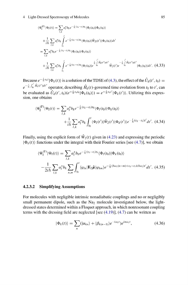
Because e
−
i
ε k t
| k (t) is a solution of the TDSE of (4.3), the effect of the ˆ
U d (t
, t 0 ) =
e
−
i
t
t 0
ˆ
H d (t
)dt
operator, describing ˆ
H d (t)-governed time evolution from t 0 to t
, can
be evaluated as ˆ
U d (t
, t 0 )(e
−
i
ε k t 0 | k (t 0 )) = e
−
i
ε k t
| k (t
). Utilizing this expression, one obtains
(F)
I | I (t) =
l,k
a ∗
l b k e −
i
(ε k −ε l )t 0 l (t 0 )| k (t 0 )
+
1
i
l,k
a ∗
l b k
t
t 0
l (t )| ˆ
W 2 (t )| k (t )e −
i
(ε k −ε l )t
dt . (4.34)
Finally, using the explicit form of ˆ
W 2 (t) given in (4.23) and expressing the periodic
| k (t) functions under the integral with their Fourier series [see (4.7)], we obtain
(F)
I | I (t) =
l,k
a
∗
l b k e
−
i
(ε k −ε l )t 0 l (t 0 )| k (t 0 )
−
1
2i
l,k
a
∗
l b k
n,m
t
t 0
ϕ ln |E 2 ˆ
μ|ϕ km e
−
i
(ω 1 (n−m)+ε k −ε l ±ω 2 )t
dt
. (4.35)
4.2.3.2 Simplifying Assumptions
For molecules with negligible intrinsic nonadiabatic couplings and no or negligibly
small permanent dipole, such as the Na 2 molecule investigated below, the lightdressed states determined within a Floquet approach, in which nonresonant coupling
terms with the dressing field are neglected [see (4.19)], (4.7) can be written as
| k (t) =
n
(|α kn + |β k(n−1) e
−iω 1 t
)e
inω 1 t
,
(4.36)
85
(F)
I | I (t) =
l,k
a
∗
l b k e
−
i
(εk −εl )t0 l (t 0 )| k (t 0 )
+
1
i
l,k
a
∗
l b k
t
t0
e
−
i
(εk −εl )t0 l (t 0 )| ˆ
W 2I (t
)| k (t 0 )dt
=
l,k
a
∗
l b k e
−
i
(εk −εl )t0 l (t 0 )| k (t 0 )
+
1
i
l,k
a
∗
l b k
t
t0
e
−
i
(εk −εl )t0 l (t 0 )|e
i
t
t 0
ˆ
Hd (t )dt
ˆ
W 2 (t
)e
−
i
t
t 0
ˆ
Hd (t )dt
| k (t 0 )dt
. (4.33)
Because e
−
i
ε k t
| k (t) is a solution of the TDSE of (4.3), the effect of the ˆ
U d (t
, t 0 ) =
e
−
i
t
t 0
ˆ
H d (t
)dt
operator, describing ˆ
H d (t)-governed time evolution from t 0 to t
, can
be evaluated as ˆ
U d (t
, t 0 )(e
−
i
ε k t 0 | k (t 0 )) = e
−
i
ε k t
| k (t
). Utilizing this expression, one obtains
(F)
I | I (t) =
l,k
a ∗
l b k e −
i
(ε k −ε l )t 0 l (t 0 )| k (t 0 )
+
1
i
l,k
a ∗
l b k
t
t 0
l (t )| ˆ
W 2 (t )| k (t )e −
i
(ε k −ε l )t
dt . (4.34)
Finally, using the explicit form of ˆ
W 2 (t) given in (4.23) and expressing the periodic
| k (t) functions under the integral with their Fourier series [see (4.7)], we obtain
(F)
I | I (t) =
l,k
a
∗
l b k e
−
i
(ε k −ε l )t 0 l (t 0 )| k (t 0 )
−
1
2i
l,k
a
∗
l b k
n,m
t
t 0
ϕ ln |E 2 ˆ
μ|ϕ km e
−
i
(ω 1 (n−m)+ε k −ε l ±ω 2 )t
dt
. (4.35)
4.2.3.2 Simplifying Assumptions
For molecules with negligible intrinsic nonadiabatic couplings and no or negligibly
small permanent dipole, such as the Na 2 molecule investigated below, the lightdressed states determined within a Floquet approach, in which nonresonant coupling
terms with the dressing field are neglected [see (4.19)], (4.7) can be written as
| k (t) =
n
(|α kn + |β k(n−1) e
−iω 1 t
)e
inω 1 t
,
(4.36)