

4 Light-Dressed Spectroscopy of Molecules
81
where
(H F ) mα v J ,nαv J
=
α
v
J
| ˆ
H mol |αv J + mω 1 δ αα δ vv δ J J
δ nm
−
1
2
α
v
J
|E 1 ˆ
μ|αv J
δ n,m−1 + δ n,m+1
.
(4.12)
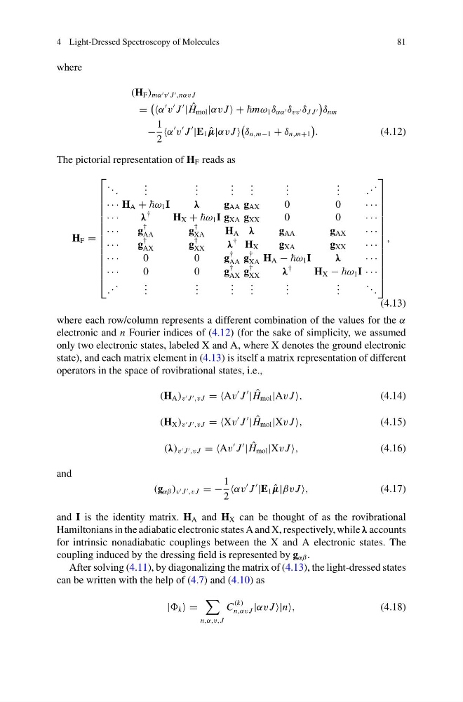
The pictorial representation of H F reads as
H F =
⎡
⎢
⎢
⎢
⎢
⎢
⎢
⎢
⎢
⎢
⎢
⎢
⎢
⎢
⎣
. . .
. . .
. . .
. . .
. . .
. . .
. . .
.
.
.
· · · H A + ω 1 I
λ
g AA g AX
0
0
· · ·
· · ·
λ
†
H X + ω 1 I g XA g XX
0
0
· · ·
· · ·
g
†
AA
g
†
XA
H A λ
g AA
g AX
· · ·
· · ·
g
†
AX
g
†
XX
λ
† H X
g XA
g XX
· · ·
· · ·
0
0
g
†
AA g
†
XA H A − ω 1 I
λ
· · ·
· · ·
0
0
g
†
AX g
†
XX
λ
†
H X − ω 1 I · · ·
.
.
.
. . .
. . .
. . .
. . .
. . .
. . .
. . .
⎤
⎥
⎥
⎥
⎥
⎥
⎥
⎥
⎥
⎥
⎥
⎥
⎥
⎥
⎦
,
(4.13)
where each row/column represents a different combination of the values for the α
electronic and n Fourier indices of (4.12) (for the sake of simplicity, we assumed
only two electronic states, labeled X and A, where X denotes the ground electronic
state), and each matrix element in (4.13) is itself a matrix representation of different
operators in the space of rovibrational states, i.e.,
(H A ) v J ,v J = =Av
J
| ˆ
H mol |Av J ,
(4.14)
(H X ) v J ,v J = =Xv
J
| ˆ
H mol |Xv J ,
(4.15)
(λ) v J ,v J = =Av
J
| ˆ
H mol |Xv J ,
(4.16)
and
(g αβ ) v J ,v J = −
1
2
αv
J
|E 1 ˆ
μ|βv J ,
(4.17)
and I is the identity matrix. H A and H X can be thought of as the rovibrational
Hamiltonians in the adiabatic electronic states A and X, respectively, while λ accounts
for intrinsic nonadiabatic couplings between the X and A electronic states. The
coupling induced by the dressing field is represented by g αβ .
After solving (4.11), by diagonalizing the matrix of (4.13), the light-dressed states
can be written with the help of (4.7) and (4.10) as
| k =
n,α,v,J
C
(k)
n,αv J |αv J |n,
(4.18)
81
where
(H F ) mα v J ,nαv J
=
α
v
J
| ˆ
H mol |αv J + mω 1 δ αα δ vv δ J J
δ nm
−
1
2
α
v
J
|E 1 ˆ
μ|αv J
δ n,m−1 + δ n,m+1
.
(4.12)
The pictorial representation of H F reads as
H F =
⎡
⎢
⎢
⎢
⎢
⎢
⎢
⎢
⎢
⎢
⎢
⎢
⎢
⎢
⎣
. . .
. . .
. . .
. . .
. . .
. . .
. . .
.
.
.
· · · H A + ω 1 I
λ
g AA g AX
0
0
· · ·
· · ·
λ
†
H X + ω 1 I g XA g XX
0
0
· · ·
· · ·
g
†
AA
g
†
XA
H A λ
g AA
g AX
· · ·
· · ·
g
†
AX
g
†
XX
λ
† H X
g XA
g XX
· · ·
· · ·
0
0
g
†
AA g
†
XA H A − ω 1 I
λ
· · ·
· · ·
0
0
g
†
AX g
†
XX
λ
†
H X − ω 1 I · · ·
.
.
.
. . .
. . .
. . .
. . .
. . .
. . .
. . .
⎤
⎥
⎥
⎥
⎥
⎥
⎥
⎥
⎥
⎥
⎥
⎥
⎥
⎥
⎦
,
(4.13)
where each row/column represents a different combination of the values for the α
electronic and n Fourier indices of (4.12) (for the sake of simplicity, we assumed
only two electronic states, labeled X and A, where X denotes the ground electronic
state), and each matrix element in (4.13) is itself a matrix representation of different
operators in the space of rovibrational states, i.e.,
(H A ) v J ,v J = =Av
J
| ˆ
H mol |Av J ,
(4.14)
(H X ) v J ,v J = =Xv
J
| ˆ
H mol |Xv J ,
(4.15)
(λ) v J ,v J = =Av
J
| ˆ
H mol |Xv J ,
(4.16)
and
(g αβ ) v J ,v J = −
1
2
αv
J
|E 1 ˆ
μ|βv J ,
(4.17)
and I is the identity matrix. H A and H X can be thought of as the rovibrational
Hamiltonians in the adiabatic electronic states A and X, respectively, while λ accounts
for intrinsic nonadiabatic couplings between the X and A electronic states. The
coupling induced by the dressing field is represented by g αβ .
After solving (4.11), by diagonalizing the matrix of (4.13), the light-dressed states
can be written with the help of (4.7) and (4.10) as
| k =
n,α,v,J
C
(k)
n,αv J |αv J |n,
(4.18)