

560
6 Reverse Engineering of Microcircuits
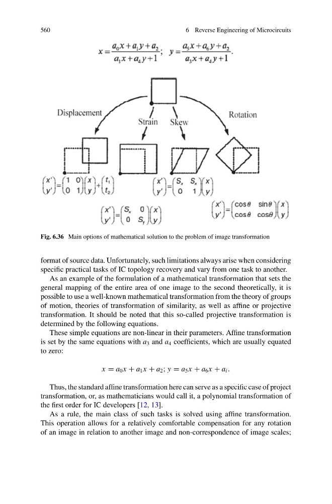
Fig. 6.36 Main options of mathematical solution to the problem of image transformation
format of source data. Unfortunately, such limitations always arise when considering
specific practical tasks of IC topology recovery and vary from one task to another.
As an example of the formulation of a mathematical transformation that sets the
general mapping of the entire area of one image to the second theoretically, it is
possible to use a well-known mathematical transformation from the theory of groups
of motion, theories of transformation of similarity, as well as affine or projective
transformation. It should be noted that this so-called projective transformation is
determined by the following equations.
These simple equations are non-linear in their parameters. Affine transformation
is set by the same equations with a 3 and a 4 coefficients, which are usually equated
to zero:
x = a 0 x + a 1 x + a 2 ; y = a 5 x + a 6 x + a i .
Thus, the standard affine transformation here can serve as a specific case of project
transformation, or, as mathematicians would call it, a polynomial transformation of
the first order for IC developers [12, 13].
As a rule, the main class of such tasks is solved using affine transformation.
This operation allows for a relatively comfortable compensation for any rotation
of an image in relation to another image and non-correspondence of image scales;
6 Reverse Engineering of Microcircuits
Fig. 6.36 Main options of mathematical solution to the problem of image transformation
format of source data. Unfortunately, such limitations always arise when considering
specific practical tasks of IC topology recovery and vary from one task to another.
As an example of the formulation of a mathematical transformation that sets the
general mapping of the entire area of one image to the second theoretically, it is
possible to use a well-known mathematical transformation from the theory of groups
of motion, theories of transformation of similarity, as well as affine or projective
transformation. It should be noted that this so-called projective transformation is
determined by the following equations.
These simple equations are non-linear in their parameters. Affine transformation
is set by the same equations with a 3 and a 4 coefficients, which are usually equated
to zero:
x = a 0 x + a 1 x + a 2 ; y = a 5 x + a 6 x + a i .
Thus, the standard affine transformation here can serve as a specific case of project
transformation, or, as mathematicians would call it, a polynomial transformation of
the first order for IC developers [12, 13].
As a rule, the main class of such tasks is solved using affine transformation.
This operation allows for a relatively comfortable compensation for any rotation
of an image in relation to another image and non-correspondence of image scales;