

Automated Upgraded Generalized Full-Discretization Method …
99
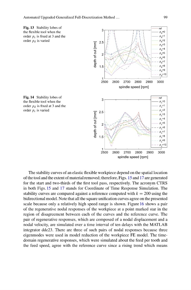
Fig. 13 Stability lobes of
the flexible tool when the
order p c is fixed at 3 and the
order p d is varied
2500 2600 2700 2800 2900 3000
spindle speed [rpm]
1
1.5
2
2.5
3
depth of cut [mm]
ref
p d =0
p d =1
p d =2
p d =3
p d =4
p d =5
p d =6
p d =7
p d =8
p d =9
p d =10
Fig. 14 Stability lobes of
the flexible tool when the
order p d is fixed at 3 and the
order p c is varied
2500 2600 2700 2800 2900 3000
spindle speed [rpm]
1
1.5
2
2.5
3
depth of cut [mm]
ref
p c =0
p c =1
p c =2
p c =3
p c =4
p c =5
p c =6
p c =7
p c =8
p c =9
p c =10
The stability curves of an elastic flexible workpiece depend on the spatial location
of the tool and the extent of material removed; therefore, Figs. 15 and 17 are generated
for the start and two-thirds of the first tool pass, respectively. The acronym CTRS
in both Figs. 15 and 17 stands for Coordinate of Time Response Simulation. The
stability curves are compared against a reference computed with k = 200 using the
bidirectional model. Note that all the square unification curves agree on the presented
scale because only a relatively high speed range is shown. Figure 16 shows a pair
of the regenerative nodal responses of the workpiece at a point marked star in the
region of disagreement between each of the curves and the reference curve. The
pair of regenerative responses, which are composed of a nodal displacement and a
nodal velocity, are simulated over a time interval of ten delays with the MATLAB
integrator dde23. There are three of such pairs of nodal responses because three
eigenmodes were used in model reduction of the workpiece FE model. The timedomain regenerative responses, which were simulated about the feed per tooth and
the feed speed, agree with the reference curve since a rising trend which means
99
Fig. 13 Stability lobes of
the flexible tool when the
order p c is fixed at 3 and the
order p d is varied
2500 2600 2700 2800 2900 3000
spindle speed [rpm]
1
1.5
2
2.5
3
depth of cut [mm]
ref
p d =0
p d =1
p d =2
p d =3
p d =4
p d =5
p d =6
p d =7
p d =8
p d =9
p d =10
Fig. 14 Stability lobes of
the flexible tool when the
order p d is fixed at 3 and the
order p c is varied
2500 2600 2700 2800 2900 3000
spindle speed [rpm]
1
1.5
2
2.5
3
depth of cut [mm]
ref
p c =0
p c =1
p c =2
p c =3
p c =4
p c =5
p c =6
p c =7
p c =8
p c =9
p c =10
The stability curves of an elastic flexible workpiece depend on the spatial location
of the tool and the extent of material removed; therefore, Figs. 15 and 17 are generated
for the start and two-thirds of the first tool pass, respectively. The acronym CTRS
in both Figs. 15 and 17 stands for Coordinate of Time Response Simulation. The
stability curves are compared against a reference computed with k = 200 using the
bidirectional model. Note that all the square unification curves agree on the presented
scale because only a relatively high speed range is shown. Figure 16 shows a pair
of the regenerative nodal responses of the workpiece at a point marked star in the
region of disagreement between each of the curves and the reference curve. The
pair of regenerative responses, which are composed of a nodal displacement and a
nodal velocity, are simulated over a time interval of ten delays with the MATLAB
integrator dde23. There are three of such pairs of nodal responses because three
eigenmodes were used in model reduction of the workpiece FE model. The timedomain regenerative responses, which were simulated about the feed per tooth and
the feed speed, agree with the reference curve since a rising trend which means