

90
C. Ozoegwu and P. Eberhard
x i+1 = e
At x i +
t i+1
t i
e
A(t i+1 −t)
(B(t)x(t) − B(t)x(t − τ ))dt.
(16)
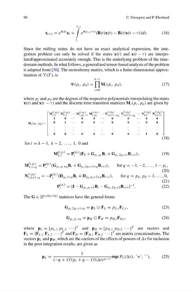
Since the milling states do not have an exact analytical expression, the integration problem can only be solved if the states x(t) and x(t − τ ) are interpolated/approximated accurately enough. This is the underlying problem of the timedomain methods. In what follows, a generalized tensor-based analysis of the problem
is adapted from [30]. The monodromy matrix, which is a finite-dimensional approximation of ϒ(T ), is
( p c , p d ) =
k−1
i=0
M i ( p c , p d ),
(17)
where p c and p d are the degrees of the respective polynomials interpolating the states
x(t) and x(t − τ ) and the discrete time transition matrices M i ( p c , p d ) are given by
M i ( p c , p d ) =
⎡
⎢
⎢
⎢
⎢
⎢
⎢
⎢
⎣
M
(i, pc )
1,1
M
(i, pc )
1,2
· · · M
(i, pc )
1, pc −1 M
(i, pc )
1, pc · · · N
(i, p d )
1,k+1− p d
N
(i, p d )
1,k+2− p d
· · · N
(i, p d )
1,k
N
(i, p d )
1,k+1
I
0
· · ·
0
0
· · ·
0
0
· · ·
0
0
0
I
· · ·
0
0
· · ·
0
0
· · ·
0
0
.
.
.
.
.
.
.
.
.
.
.
.
.
.
.
.
.
.
.
.
.
.
.
.
.
.
.
.
.
.
.
.
.
0
0
· · ·
0
0
· · ·
0
0
· · ·
I
0
⎤
⎥
⎥
⎥
⎥
⎥
⎥
⎥
⎦
(18)
for i = k − 1, k − 2, . . . , 1, 0 and
M
(i, p c )
1,1
= P
( p c )
i
(F 0 + G p c , p c B i + G p c ,2 p c +1 B i+1 ),
(19)
M
(i, p c )
1,1−q = P
( p c )
i
(G p c , p c +q B i + G p c ,2 p c +1+q B i+1 ),
for q = −1, −2, . . . , 1 − p c ,
(20)
N
(i, p d )
1,k+1−q = −P
( p c )
i
(D p d ,1+q B i + D p d , p d +2+q B i+1 ),
for q = p d , p d − 1, . . . , 0,
(21)
P
( p c )
i
= [I − G p c , p c +1 B i − G p c ,2 p c +2 B i+1 ]
−1
.
(22)
The G ∈ R
n d (d R ×d R ) matrices have the general forms
G p c ,2 p c +1+q = p L F L = p L ,i F L ,i ,
(23)
G p c , p c +q = p H F H = p H,i F H,i ,
(24)
where p L = {p L ,1 p L ,2 · · · }
T and p H = {p H,1 p H,2 · · · }
T are vectors and
F L = {F L ,1 F L ,2 · · · }
T and F H = {F H,1 F H,2 · · · }
T are matrix concatenations. The
vectors p L and p H , which are the carriers of the effects of powers of t for inclusion
in the post-integration results, are given as
p L =
1
(−q + 1)!( p c + q − 1)!((t) p c +1 rep(P L ((t),
+
,
),
(25)
C. Ozoegwu and P. Eberhard
x i+1 = e
At x i +
t i+1
t i
e
A(t i+1 −t)
(B(t)x(t) − B(t)x(t − τ ))dt.
(16)
Since the milling states do not have an exact analytical expression, the integration problem can only be solved if the states x(t) and x(t − τ ) are interpolated/approximated accurately enough. This is the underlying problem of the timedomain methods. In what follows, a generalized tensor-based analysis of the problem
is adapted from [30]. The monodromy matrix, which is a finite-dimensional approximation of ϒ(T ), is
( p c , p d ) =
k−1
i=0
M i ( p c , p d ),
(17)
where p c and p d are the degrees of the respective polynomials interpolating the states
x(t) and x(t − τ ) and the discrete time transition matrices M i ( p c , p d ) are given by
M i ( p c , p d ) =
⎡
⎢
⎢
⎢
⎢
⎢
⎢
⎢
⎣
M
(i, pc )
1,1
M
(i, pc )
1,2
· · · M
(i, pc )
1, pc −1 M
(i, pc )
1, pc · · · N
(i, p d )
1,k+1− p d
N
(i, p d )
1,k+2− p d
· · · N
(i, p d )
1,k
N
(i, p d )
1,k+1
I
0
· · ·
0
0
· · ·
0
0
· · ·
0
0
0
I
· · ·
0
0
· · ·
0
0
· · ·
0
0
.
.
.
.
.
.
.
.
.
.
.
.
.
.
.
.
.
.
.
.
.
.
.
.
.
.
.
.
.
.
.
.
.
0
0
· · ·
0
0
· · ·
0
0
· · ·
I
0
⎤
⎥
⎥
⎥
⎥
⎥
⎥
⎥
⎦
(18)
for i = k − 1, k − 2, . . . , 1, 0 and
M
(i, p c )
1,1
= P
( p c )
i
(F 0 + G p c , p c B i + G p c ,2 p c +1 B i+1 ),
(19)
M
(i, p c )
1,1−q = P
( p c )
i
(G p c , p c +q B i + G p c ,2 p c +1+q B i+1 ),
for q = −1, −2, . . . , 1 − p c ,
(20)
N
(i, p d )
1,k+1−q = −P
( p c )
i
(D p d ,1+q B i + D p d , p d +2+q B i+1 ),
for q = p d , p d − 1, . . . , 0,
(21)
P
( p c )
i
= [I − G p c , p c +1 B i − G p c ,2 p c +2 B i+1 ]
−1
.
(22)
The G ∈ R
n d (d R ×d R ) matrices have the general forms
G p c ,2 p c +1+q = p L F L = p L ,i F L ,i ,
(23)
G p c , p c +q = p H F H = p H,i F H,i ,
(24)
where p L = {p L ,1 p L ,2 · · · }
T and p H = {p H,1 p H,2 · · · }
T are vectors and
F L = {F L ,1 F L ,2 · · · }
T and F H = {F H,1 F H,2 · · · }
T are matrix concatenations. The
vectors p L and p H , which are the carriers of the effects of powers of t for inclusion
in the post-integration results, are given as
p L =
1
(−q + 1)!( p c + q − 1)!((t) p c +1 rep(P L ((t),
+
,
),
(25)