

Automated Upgraded Generalized Full-Discretization Method …
89
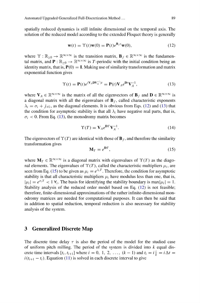
spatially reduced dynamics is still infinite dimensional on the temporal axis. The
solution of the reduced model according to the extended Floquet theory is generally
w(t) = ϒ(t)w(0) = P(t)e
B f t w(0),
(12)
where ϒ : R ≥0 → R
∞×∞ is the transition matrix, B f ∈ R
∞×∞ is the fundamental matrix, and P : R ≥0 → R
∞×∞ is T -periodic with the initial condition being an
identity matrix, that is, P(0) = I. Making use of similarity transformation and matrix
exponential function gives
ϒ(t) = P(t)e
(V A DV
−1
A )t
= P(t)V A e
Dt V
−1
A ,
(13)
where V A ∈ R
∞×∞ is the matrix of all the eigenvectors of B f and D ∈ R
∞×∞ is
a diagonal matrix with all the eigenvalues of B f , called characteristic exponents
λ i = σ i + jω i , as the diagonal elements. It is obvious from Eqs. (12) and (13) that
the condition for asymptotic stability is that all λ i have negative real parts, that is,
σ i < 0. From Eq. (13), the monodromy matrix becomes
ϒ(T ) = V A e
DT V
−1
A .
(14)
The eigenvectors of ϒ(T ) are identical with those of B f , and therefore the similarity
transformation gives
M T = e
DT
,
(15)
where M T ∈ R
∞×∞ is a diagonal matrix with eigenvalues of ϒ(T ) as the diagonal elements. The eigenvalues of ϒ(T ), called the characteristic multipliers μ i , are
seen from Eq. (15) to be given as μ i = e
λ i T . Therefore, the condition for asymptotic
stability is that all characteristic multipliers μ i have modulus less than one, that is,
|μ i | = e
σ i T
< 1 ∀ i . The basis for identifying the stability boundary is max|μ i | = 1.
Stability analysis of the reduced order model based on Eq. (12) is not feasible;
therefore, finite-dimensional approximations of the rather infinite-dimensional monodromy matrices are needed for computational purposes. It can then be said that
in addition to spatial reduction, temporal reduction is also necessary for stability
analysis of the system.
3 Generalized Discrete Map
The discrete time delay τ is also the period of the model for the studied case
of uniform pitch milling. The period of the system is divided into k equal discrete time intervals [t i , t i+1 ] where i = 0, 1, 2, . . . , (k − 1) and t i = i
τ
k
= it =
i(t i+1 − t i ). Equation (11) is solved in each discrete interval to give
89
spatially reduced dynamics is still infinite dimensional on the temporal axis. The
solution of the reduced model according to the extended Floquet theory is generally
w(t) = ϒ(t)w(0) = P(t)e
B f t w(0),
(12)
where ϒ : R ≥0 → R
∞×∞ is the transition matrix, B f ∈ R
∞×∞ is the fundamental matrix, and P : R ≥0 → R
∞×∞ is T -periodic with the initial condition being an
identity matrix, that is, P(0) = I. Making use of similarity transformation and matrix
exponential function gives
ϒ(t) = P(t)e
(V A DV
−1
A )t
= P(t)V A e
Dt V
−1
A ,
(13)
where V A ∈ R
∞×∞ is the matrix of all the eigenvectors of B f and D ∈ R
∞×∞ is
a diagonal matrix with all the eigenvalues of B f , called characteristic exponents
λ i = σ i + jω i , as the diagonal elements. It is obvious from Eqs. (12) and (13) that
the condition for asymptotic stability is that all λ i have negative real parts, that is,
σ i < 0. From Eq. (13), the monodromy matrix becomes
ϒ(T ) = V A e
DT V
−1
A .
(14)
The eigenvectors of ϒ(T ) are identical with those of B f , and therefore the similarity
transformation gives
M T = e
DT
,
(15)
where M T ∈ R
∞×∞ is a diagonal matrix with eigenvalues of ϒ(T ) as the diagonal elements. The eigenvalues of ϒ(T ), called the characteristic multipliers μ i , are
seen from Eq. (15) to be given as μ i = e
λ i T . Therefore, the condition for asymptotic
stability is that all characteristic multipliers μ i have modulus less than one, that is,
|μ i | = e
σ i T
< 1 ∀ i . The basis for identifying the stability boundary is max|μ i | = 1.
Stability analysis of the reduced order model based on Eq. (12) is not feasible;
therefore, finite-dimensional approximations of the rather infinite-dimensional monodromy matrices are needed for computational purposes. It can then be said that
in addition to spatial reduction, temporal reduction is also necessary for stability
analysis of the system.
3 Generalized Discrete Map
The discrete time delay τ is also the period of the model for the studied case
of uniform pitch milling. The period of the system is divided into k equal discrete time intervals [t i , t i+1 ] where i = 0, 1, 2, . . . , (k − 1) and t i = i
τ
k
= it =
i(t i+1 − t i ). Equation (11) is solved in each discrete interval to give