

464
M. N. Bojnordi and P. Behnam
A (3)
B (10)
C (6)
D (12)
E (2)
0
1
0
1
0
0
0
1
1
0
1
1
1
0
1
1
0
0
0
0
:
:
:
:
:
Median
? ? ? ?
:
A (0.4)
B (1.2)
C (0.8)
D (1.5)
E (0.25)
A (3)
B (10)
C (6)
D (12)
E (2)
0
1
0
1
0
0
0
1
1
0
1
1
1
0
1
1
0
0
0
0
:
:
:
:
:
Median
0 1 1 0
:
Bit-serial Median
Computation
2 3
A (0.4)
B (1.2)
C (0.8)
D (1.5)
E (0.25)
Fig. 9.27 Illustrative example of handling real valued numbers in the MISC framework
A (5)
B (1)
C (2)
D (9)
E (10)
0
0
0
1
1
1
0
0
0
0
0
0
1
0
1
1
1
0
1
0
:
:
:
:
:
Median
? ? ? ?
:
A (-3)
B (-7)
C (-6)
D (1)
E (2)
Bit-serial Median
Computation
2 3
A (5)
B (1)
C (2)
D (9)
E (10)
0
0
0
1
1
1
0
0
0
0
0
0
1
0
1
1
1
0
1
0
:
:
:
:
:
Median
0 1 0 1
:
A (-3)
B (-7)
C (-6)
D (1)
E (2)
Fig. 9.28 Illustrative example of handling negative numbers in the MISC framework
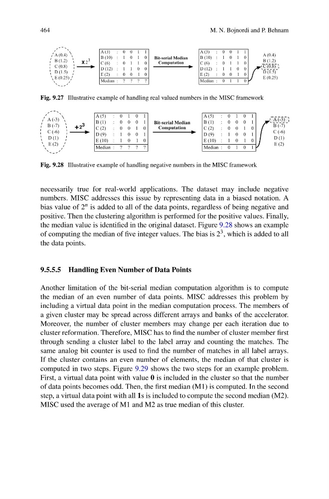
necessarily true for real-world applications. The dataset may include negative
numbers. MISC addresses this issue by representing data in a biased notation. A
bias value of 2 n is added to all of the data points, regardless of being negative and
positive. Then the clustering algorithm is performed for the positive values. Finally,
the median value is identified in the original dataset. Figure 9.28 shows an example
of computing the median of five integer values. The bias is 2 3 , which is added to all
the data points.
9.5.5.5 Handling Even Number of Data Points
Another limitation of the bit-serial median computation algorithm is to compute
the median of an even number of data points. MISC addresses this problem by
including a virtual data point in the median computation process. The members of
a given cluster may be spread across different arrays and banks of the accelerator.
Moreover, the number of cluster members may change per each iteration due to
cluster reformation. Therefore, MISC has to find the number of cluster member first
through sending a cluster label to the label array and counting the matches. The
same analog bit counter is used to find the number of matches in all label arrays.
If the cluster contains an even number of elements, the median of that cluster is
computed in two steps. Figure 9.29 shows the two steps for an example problem.
First, a virtual data point with value 0 is included in the cluster so that the number
of data points becomes odd. Then, the first median (M1) is computed. In the second
step, a virtual data point with all 1s is included to compute the second median (M2).
MISC used the average of M1 and M2 as true median of this cluster.
M. N. Bojnordi and P. Behnam
A (3)
B (10)
C (6)
D (12)
E (2)
0
1
0
1
0
0
0
1
1
0
1
1
1
0
1
1
0
0
0
0
:
:
:
:
:
Median
? ? ? ?
:
A (0.4)
B (1.2)
C (0.8)
D (1.5)
E (0.25)
A (3)
B (10)
C (6)
D (12)
E (2)
0
1
0
1
0
0
0
1
1
0
1
1
1
0
1
1
0
0
0
0
:
:
:
:
:
Median
0 1 1 0
:
Bit-serial Median
Computation
2 3
A (0.4)
B (1.2)
C (0.8)
D (1.5)
E (0.25)
Fig. 9.27 Illustrative example of handling real valued numbers in the MISC framework
A (5)
B (1)
C (2)
D (9)
E (10)
0
0
0
1
1
1
0
0
0
0
0
0
1
0
1
1
1
0
1
0
:
:
:
:
:
Median
? ? ? ?
:
A (-3)
B (-7)
C (-6)
D (1)
E (2)
Bit-serial Median
Computation
2 3
A (5)
B (1)
C (2)
D (9)
E (10)
0
0
0
1
1
1
0
0
0
0
0
0
1
0
1
1
1
0
1
0
:
:
:
:
:
Median
0 1 0 1
:
A (-3)
B (-7)
C (-6)
D (1)
E (2)
Fig. 9.28 Illustrative example of handling negative numbers in the MISC framework
necessarily true for real-world applications. The dataset may include negative
numbers. MISC addresses this issue by representing data in a biased notation. A
bias value of 2 n is added to all of the data points, regardless of being negative and
positive. Then the clustering algorithm is performed for the positive values. Finally,
the median value is identified in the original dataset. Figure 9.28 shows an example
of computing the median of five integer values. The bias is 2 3 , which is added to all
the data points.
9.5.5.5 Handling Even Number of Data Points
Another limitation of the bit-serial median computation algorithm is to compute
the median of an even number of data points. MISC addresses this problem by
including a virtual data point in the median computation process. The members of
a given cluster may be spread across different arrays and banks of the accelerator.
Moreover, the number of cluster members may change per each iteration due to
cluster reformation. Therefore, MISC has to find the number of cluster member first
through sending a cluster label to the label array and counting the matches. The
same analog bit counter is used to find the number of matches in all label arrays.
If the cluster contains an even number of elements, the median of that cluster is
computed in two steps. Figure 9.29 shows the two steps for an example problem.
First, a virtual data point with value 0 is included in the cluster so that the number
of data points becomes odd. Then, the first median (M1) is computed. In the second
step, a virtual data point with all 1s is included to compute the second median (M2).
MISC used the average of M1 and M2 as true median of this cluster.