

5 Machine Learning for IoT
309
Input: 6*6*3
Filter: 3*3*3
Output: 4*4*1
=
*
Input: 6*6*3
Filter: 3*3*3
Output: 4*4*1
=
*
Input: 6*6*3
Filter: 3*3*3
Output: 4*4*1
=
*
Final: 4*4*3
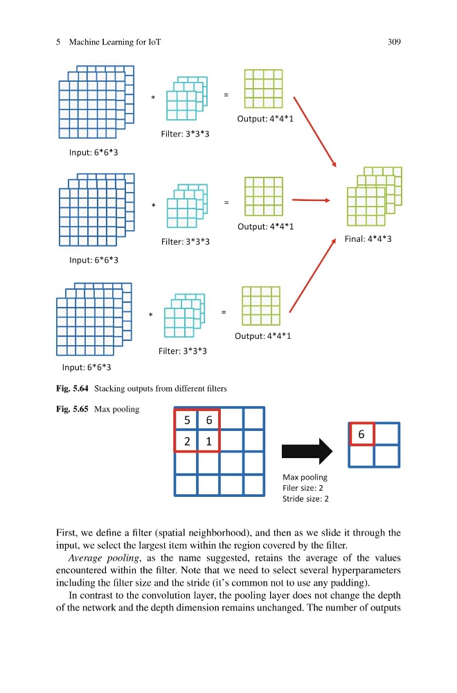
Fig. 5.64 Stacking outputs from different filters
Fig. 5.65 Max pooling
Max pooling
Filer size: 2
Stride size: 2
5 6
2 1
6
First, we define a filter (spatial neighborhood), and then as we slide it through the
input, we select the largest item within the region covered by the filter.
Average pooling, as the name suggested, retains the average of the values
encountered within the filter. Note that we need to select several hyperparameters
including the filter size and the stride (it’s common not to use any padding).
In contrast to the convolution layer, the pooling layer does not change the depth
of the network and the depth dimension remains unchanged. The number of outputs
309
Input: 6*6*3
Filter: 3*3*3
Output: 4*4*1
=
*
Input: 6*6*3
Filter: 3*3*3
Output: 4*4*1
=
*
Input: 6*6*3
Filter: 3*3*3
Output: 4*4*1
=
*
Final: 4*4*3
Fig. 5.64 Stacking outputs from different filters
Fig. 5.65 Max pooling
Max pooling
Filer size: 2
Stride size: 2
5 6
2 1
6
First, we define a filter (spatial neighborhood), and then as we slide it through the
input, we select the largest item within the region covered by the filter.
Average pooling, as the name suggested, retains the average of the values
encountered within the filter. Note that we need to select several hyperparameters
including the filter size and the stride (it’s common not to use any padding).
In contrast to the convolution layer, the pooling layer does not change the depth
of the network and the depth dimension remains unchanged. The number of outputs