

308
F. Firouzi et al.
Input: 6*6*3
Filter: 3*3*3
Output: 4*4*1
=
*
should be equal
#Channel
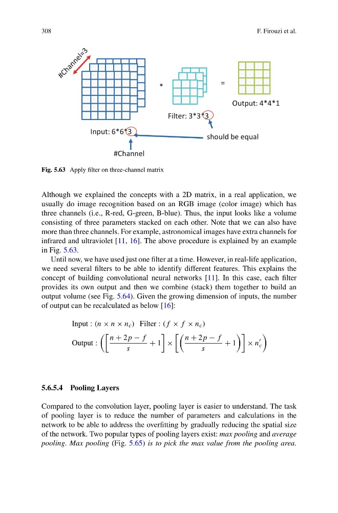
Fig. 5.63 Apply filter on three-channel matrix
Although we explained the concepts with a 2D matrix, in a real application, we
usually do image recognition based on an RGB image (color image) which has
three channels (i.e., R-red, G-green, B-blue). Thus, the input looks like a volume
consisting of three parameters stacked on each other. Note that we can also have
more than three channels. For example, astronomical images have extra channels for
infrared and ultraviolet [11, 16]. The above procedure is explained by an example
in Fig. 5.63.
Until now, we have used just one filter at a time. However, in real-life application,
we need several filters to be able to identify different features. This explains the
concept of building convolutional neural networks [11]. In this case, each filter
provides its own output and then we combine (stack) them together to build an
output volume (see Fig. 5.64). Given the growing dimension of inputs, the number
of output can be recalculated as below [16]:
Input : (n × n × n c ) Filter : (f × f × n c )
Output :
n + 2p − f
s
+ 1
×
n + 2p − f
s
+ 1
× n
c
5.6.5.4 Pooling Layers
Compared to the convolution layer, pooling layer is easier to understand. The task
of pooling layer is to reduce the number of parameters and calculations in the
network to be able to address the overfitting by gradually reducing the spatial size
of the network. Two popular types of pooling layers exist: max pooling and average
pooling. Max pooling (Fig. 5.65) is to pick the max value from the pooling area.
F. Firouzi et al.
Input: 6*6*3
Filter: 3*3*3
Output: 4*4*1
=
*
should be equal
#Channel
Fig. 5.63 Apply filter on three-channel matrix
Although we explained the concepts with a 2D matrix, in a real application, we
usually do image recognition based on an RGB image (color image) which has
three channels (i.e., R-red, G-green, B-blue). Thus, the input looks like a volume
consisting of three parameters stacked on each other. Note that we can also have
more than three channels. For example, astronomical images have extra channels for
infrared and ultraviolet [11, 16]. The above procedure is explained by an example
in Fig. 5.63.
Until now, we have used just one filter at a time. However, in real-life application,
we need several filters to be able to identify different features. This explains the
concept of building convolutional neural networks [11]. In this case, each filter
provides its own output and then we combine (stack) them together to build an
output volume (see Fig. 5.64). Given the growing dimension of inputs, the number
of output can be recalculated as below [16]:
Input : (n × n × n c ) Filter : (f × f × n c )
Output :
n + 2p − f
s
+ 1
×
n + 2p − f
s
+ 1
× n
c
5.6.5.4 Pooling Layers
Compared to the convolution layer, pooling layer is easier to understand. The task
of pooling layer is to reduce the number of parameters and calculations in the
network to be able to address the overfitting by gradually reducing the spatial size
of the network. Two popular types of pooling layers exist: max pooling and average
pooling. Max pooling (Fig. 5.65) is to pick the max value from the pooling area.