

5 Machine Learning for IoT
299
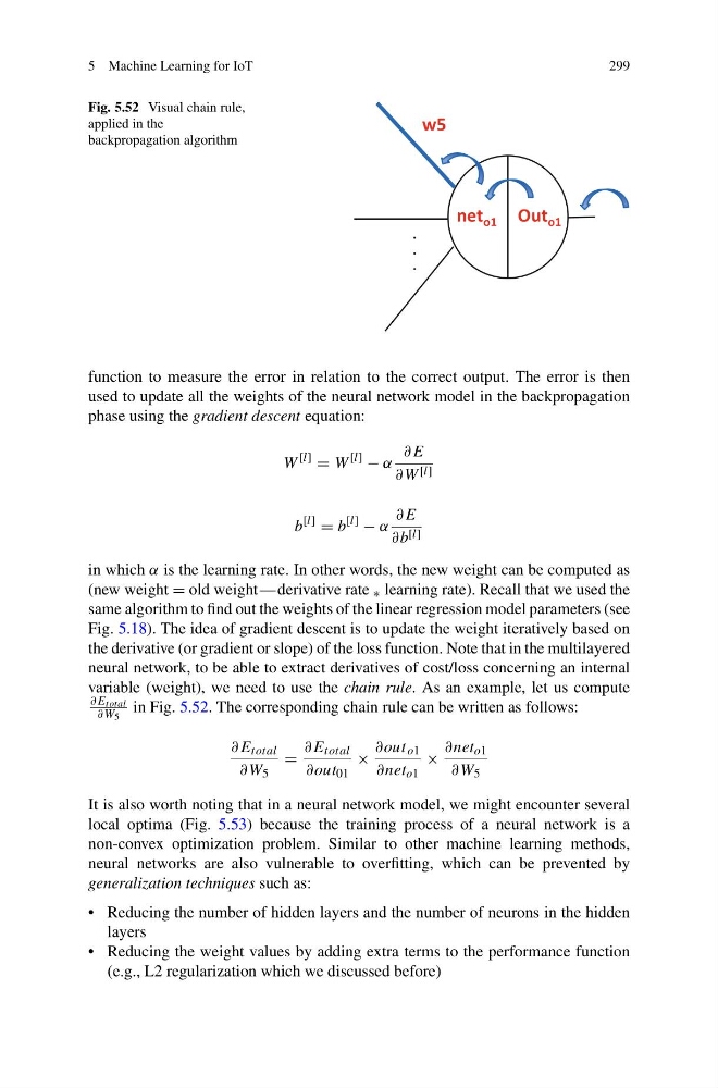
Fig. 5.52 Visual chain rule,
applied in the
backpropagation algorithm
Out o1
net o1
w5
.
.
.
function to measure the error in relation to the correct output. The error is then
used to update all the weights of the neural network model in the backpropagation
phase using the gradient descent equation:
W
[l]
= W
[l]
− α
∂E
∂W [l]
b
[l]
= b
[l]
− α
∂E
∂b [l]
in which α is the learning rate. In other words, the new weight can be computed as
(new weight = old weight — derivative rate ∗ learning rate). Recall that we used the
same algorithm to find out the weights of the linear regression model parameters (see
Fig. 5.18). The idea of gradient descent is to update the weight iteratively based on
the derivative (or gradient or slope) of the loss function. Note that in the multilayered
neural network, to be able to extract derivatives of cost/loss concerning an internal
variable (weight), we need to use the chain rule. As an example, let us compute
∂E total
∂W 5
in Fig. 5.52. The corresponding chain rule can be written as follows:
∂E total
∂W 5
=
∂E total
∂out 01
×
∂out o1
∂net o1
×
∂net o1
∂W 5
It is also worth noting that in a neural network model, we might encounter several
local optima (Fig. 5.53) because the training process of a neural network is a
non-convex optimization problem. Similar to other machine learning methods,
neural networks are also vulnerable to overfitting, which can be prevented by
generalization techniques such as:
• Reducing the number of hidden layers and the number of neurons in the hidden
layers
• Reducing the weight values by adding extra terms to the performance function
(e.g., L2 regularization which we discussed before)
299
Fig. 5.52 Visual chain rule,
applied in the
backpropagation algorithm
Out o1
net o1
w5
.
.
.
function to measure the error in relation to the correct output. The error is then
used to update all the weights of the neural network model in the backpropagation
phase using the gradient descent equation:
W
[l]
= W
[l]
− α
∂E
∂W [l]
b
[l]
= b
[l]
− α
∂E
∂b [l]
in which α is the learning rate. In other words, the new weight can be computed as
(new weight = old weight — derivative rate ∗ learning rate). Recall that we used the
same algorithm to find out the weights of the linear regression model parameters (see
Fig. 5.18). The idea of gradient descent is to update the weight iteratively based on
the derivative (or gradient or slope) of the loss function. Note that in the multilayered
neural network, to be able to extract derivatives of cost/loss concerning an internal
variable (weight), we need to use the chain rule. As an example, let us compute
∂E total
∂W 5
in Fig. 5.52. The corresponding chain rule can be written as follows:
∂E total
∂W 5
=
∂E total
∂out 01
×
∂out o1
∂net o1
×
∂net o1
∂W 5
It is also worth noting that in a neural network model, we might encounter several
local optima (Fig. 5.53) because the training process of a neural network is a
non-convex optimization problem. Similar to other machine learning methods,
neural networks are also vulnerable to overfitting, which can be prevented by
generalization techniques such as:
• Reducing the number of hidden layers and the number of neurons in the hidden
layers
• Reducing the weight values by adding extra terms to the performance function
(e.g., L2 regularization which we discussed before)