

298
F. Firouzi et al.
Input layer
Hidden layer 1
Hidden layer 2
Output layer
b
W i *x i
W 0 *x 0
From previous
neuron
x 0
W 0
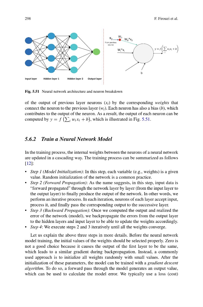
Fig. 5.51 Neural network architecture and neuron breakdown
of the output of previous layer neurons (x i ) by the corresponding weights that
connect the neuron to the previous layer (w i ). Each neuron has also a bias (b), which
contributes to the output of the neuron. As a result, the output of each neuron can be
computed by y = f
i w i x i + b
, which is illustrated in Fig. 5.51.
5.6.2 Train a Neural Network Model
In the training process, the internal weights between the neurons of a neural network
are updated in a cascading way. The training process can be summarized as follows
[12]:
• Step 1 (Model Initialization): In this step, each variable (e.g., weights) is a given
value. Random initialization of the network is a common practice.
• Step 2 (Forward Propagation): As the name suggests, in this step, input data is
“forward propagated” through the network layer by layer (from the input layer to
the output layer) to finally produce the output of the network. In other words, we
perform an iterative process. In each iteration, neurons of each layer accept input,
process it, and finally pass the corresponding output to the successive layer.
• Step 3 (Backward Propagation): Once we computed the output and realized the
error of the network (model), we backpropagate the errors from the output layer
to the hidden layers and input layer to be able to update the weights accordingly.
• Step 4: We execute steps 2 and 3 iteratively until all the weights converge.
Let us explain the above three steps in more details. Before the neural network
model training, the initial values of the weights should be selected properly. Zero is
not a good choice because it causes the output of the first layer to be the same,
which leads to a similar gradient during backpropagation. Instead, a commonly
used approach is to initialize all weights randomly with small values. After the
initialization of these parameters, the model can be trained with a gradient descent
algorithm. To do so, a forward pass through the model generates an output value,
which can be used to calculate the model error. We typically use a loss (cost)
F. Firouzi et al.
Input layer
Hidden layer 1
Hidden layer 2
Output layer
b
W i *x i
W 0 *x 0
From previous
neuron
x 0
W 0
Fig. 5.51 Neural network architecture and neuron breakdown
of the output of previous layer neurons (x i ) by the corresponding weights that
connect the neuron to the previous layer (w i ). Each neuron has also a bias (b), which
contributes to the output of the neuron. As a result, the output of each neuron can be
computed by y = f
i w i x i + b
, which is illustrated in Fig. 5.51.
5.6.2 Train a Neural Network Model
In the training process, the internal weights between the neurons of a neural network
are updated in a cascading way. The training process can be summarized as follows
[12]:
• Step 1 (Model Initialization): In this step, each variable (e.g., weights) is a given
value. Random initialization of the network is a common practice.
• Step 2 (Forward Propagation): As the name suggests, in this step, input data is
“forward propagated” through the network layer by layer (from the input layer to
the output layer) to finally produce the output of the network. In other words, we
perform an iterative process. In each iteration, neurons of each layer accept input,
process it, and finally pass the corresponding output to the successive layer.
• Step 3 (Backward Propagation): Once we computed the output and realized the
error of the network (model), we backpropagate the errors from the output layer
to the hidden layers and input layer to be able to update the weights accordingly.
• Step 4: We execute steps 2 and 3 iteratively until all the weights converge.
Let us explain the above three steps in more details. Before the neural network
model training, the initial values of the weights should be selected properly. Zero is
not a good choice because it causes the output of the first layer to be the same,
which leads to a similar gradient during backpropagation. Instead, a commonly
used approach is to initialize all weights randomly with small values. After the
initialization of these parameters, the model can be trained with a gradient descent
algorithm. To do so, a forward pass through the model generates an output value,
which can be used to calculate the model error. We typically use a loss (cost)