

5 Machine Learning for IoT
287
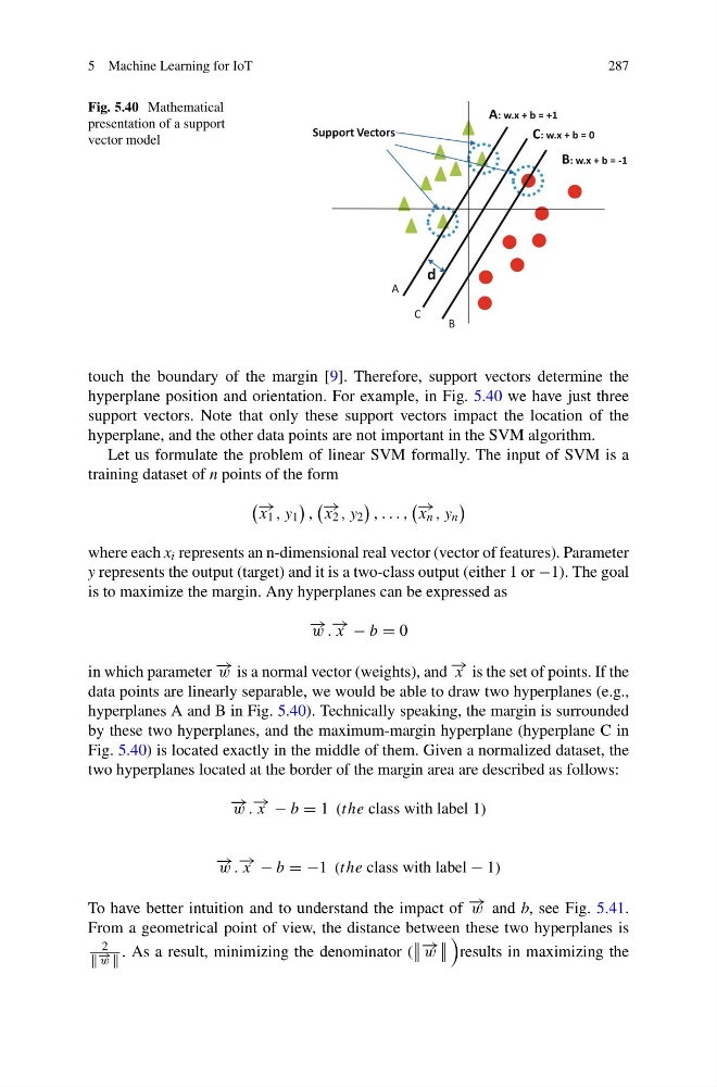
Fig. 5.40 Mathematical
presentation of a support
vector model
Support Vectors
B: w.x + b = -1
A: w.x + b = +1
C: w.x + b = 0
d
C
A
B
touch the boundary of the margin [9]. Therefore, support vectors determine the
hyperplane position and orientation. For example, in Fig. 5.40 we have just three
support vectors. Note that only these support vectors impact the location of the
hyperplane, and the other data points are not important in the SVM algorithm.
Let us formulate the problem of linear SVM formally. The input of SVM is a
training dataset of n points of the form
− → x 1 , y 1
,
− → x 2 , y 2
, . . . ,
− → x n , y n
where each x i represents an n-dimensional real vector (vector of features). Parameter
y represents the output (target) and it is a two-class output (either 1 or −1). The goal
is to maximize the margin. Any hyperplanes can be expressed as
− → w . − → x − b = 0
in which parameter − → w is a normal vector (weights), and − → x is the set of points. If the
data points are linearly separable, we would be able to draw two hyperplanes (e.g.,
hyperplanes A and B in Fig. 5.40). Technically speaking, the margin is surrounded
by these two hyperplanes, and the maximum-margin hyperplane (hyperplane C in
Fig. 5.40) is located exactly in the middle of them. Given a normalized dataset, the
two hyperplanes located at the border of the margin area are described as follows:
− → w . − → x − b = 1 (the class with label 1)
− → w . − → x − b = −1 (the class with label − 1)
To have better intuition and to understand the impact of − → w and b, see Fig. 5.41.
From a geometrical point of view, the distance between these two hyperplanes is
2
− → w
. As a result, minimizing the denominator (
− → w
results in maximizing the
287
Fig. 5.40 Mathematical
presentation of a support
vector model
Support Vectors
B: w.x + b = -1
A: w.x + b = +1
C: w.x + b = 0
d
C
A
B
touch the boundary of the margin [9]. Therefore, support vectors determine the
hyperplane position and orientation. For example, in Fig. 5.40 we have just three
support vectors. Note that only these support vectors impact the location of the
hyperplane, and the other data points are not important in the SVM algorithm.
Let us formulate the problem of linear SVM formally. The input of SVM is a
training dataset of n points of the form
− → x 1 , y 1
,
− → x 2 , y 2
, . . . ,
− → x n , y n
where each x i represents an n-dimensional real vector (vector of features). Parameter
y represents the output (target) and it is a two-class output (either 1 or −1). The goal
is to maximize the margin. Any hyperplanes can be expressed as
− → w . − → x − b = 0
in which parameter − → w is a normal vector (weights), and − → x is the set of points. If the
data points are linearly separable, we would be able to draw two hyperplanes (e.g.,
hyperplanes A and B in Fig. 5.40). Technically speaking, the margin is surrounded
by these two hyperplanes, and the maximum-margin hyperplane (hyperplane C in
Fig. 5.40) is located exactly in the middle of them. Given a normalized dataset, the
two hyperplanes located at the border of the margin area are described as follows:
− → w . − → x − b = 1 (the class with label 1)
− → w . − → x − b = −1 (the class with label − 1)
To have better intuition and to understand the impact of − → w and b, see Fig. 5.41.
From a geometrical point of view, the distance between these two hyperplanes is
2
− → w
. As a result, minimizing the denominator (
− → w
results in maximizing the