

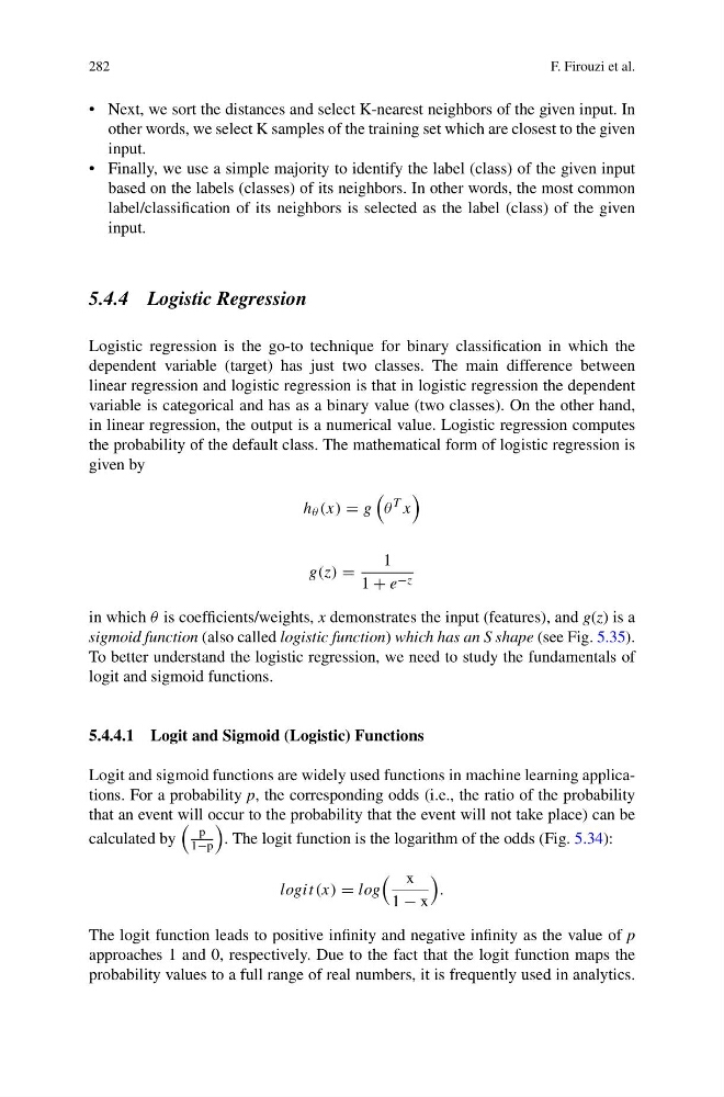
282
F. Firouzi et al.
• Next, we sort the distances and select K-nearest neighbors of the given input. In
other words, we select K samples of the training set which are closest to the given
input.
• Finally, we use a simple majority to identify the label (class) of the given input
based on the labels (classes) of its neighbors. In other words, the most common
label/classification of its neighbors is selected as the label (class) of the given
input.
5.4.4 Logistic Regression
Logistic regression is the go-to technique for binary classification in which the
dependent variable (target) has just two classes. The main difference between
linear regression and logistic regression is that in logistic regression the dependent
variable is categorical and has as a binary value (two classes). On the other hand,
in linear regression, the output is a numerical value. Logistic regression computes
the probability of the default class. The mathematical form of logistic regression is
given by
h θ (x) = g
θ
T x
g(z) =
1
1 + e −z
in which θ is coefficients/weights, x demonstrates the input (features), and g(z) is a
sigmoid function (also called logistic function) which has an S shape (see Fig. 5.35).
To better understand the logistic regression, we need to study the fundamentals of
logit and sigmoid functions.
5.4.4.1 Logit and Sigmoid (Logistic) Functions
Logit and sigmoid functions are widely used functions in machine learning applications. For a probability p, the corresponding odds (i.e., the ratio of the probability
that an event will occur to the probability that the event will not take place) can be
calculated by
p
1−p
. The logit function is the logarithm of the odds (Fig. 5.34):
logit (x) = log
x
1 − x
.
The logit function leads to positive infinity and negative infinity as the value of p
approaches 1 and 0, respectively. Due to the fact that the logit function maps the
probability values to a full range of real numbers, it is frequently used in analytics.
F. Firouzi et al.
• Next, we sort the distances and select K-nearest neighbors of the given input. In
other words, we select K samples of the training set which are closest to the given
input.
• Finally, we use a simple majority to identify the label (class) of the given input
based on the labels (classes) of its neighbors. In other words, the most common
label/classification of its neighbors is selected as the label (class) of the given
input.
5.4.4 Logistic Regression
Logistic regression is the go-to technique for binary classification in which the
dependent variable (target) has just two classes. The main difference between
linear regression and logistic regression is that in logistic regression the dependent
variable is categorical and has as a binary value (two classes). On the other hand,
in linear regression, the output is a numerical value. Logistic regression computes
the probability of the default class. The mathematical form of logistic regression is
given by
h θ (x) = g
θ
T x
g(z) =
1
1 + e −z
in which θ is coefficients/weights, x demonstrates the input (features), and g(z) is a
sigmoid function (also called logistic function) which has an S shape (see Fig. 5.35).
To better understand the logistic regression, we need to study the fundamentals of
logit and sigmoid functions.
5.4.4.1 Logit and Sigmoid (Logistic) Functions
Logit and sigmoid functions are widely used functions in machine learning applications. For a probability p, the corresponding odds (i.e., the ratio of the probability
that an event will occur to the probability that the event will not take place) can be
calculated by
p
1−p
. The logit function is the logarithm of the odds (Fig. 5.34):
logit (x) = log
x
1 − x
.
The logit function leads to positive infinity and negative infinity as the value of p
approaches 1 and 0, respectively. Due to the fact that the logit function maps the
probability values to a full range of real numbers, it is frequently used in analytics.