

5 Machine Learning for IoT
273
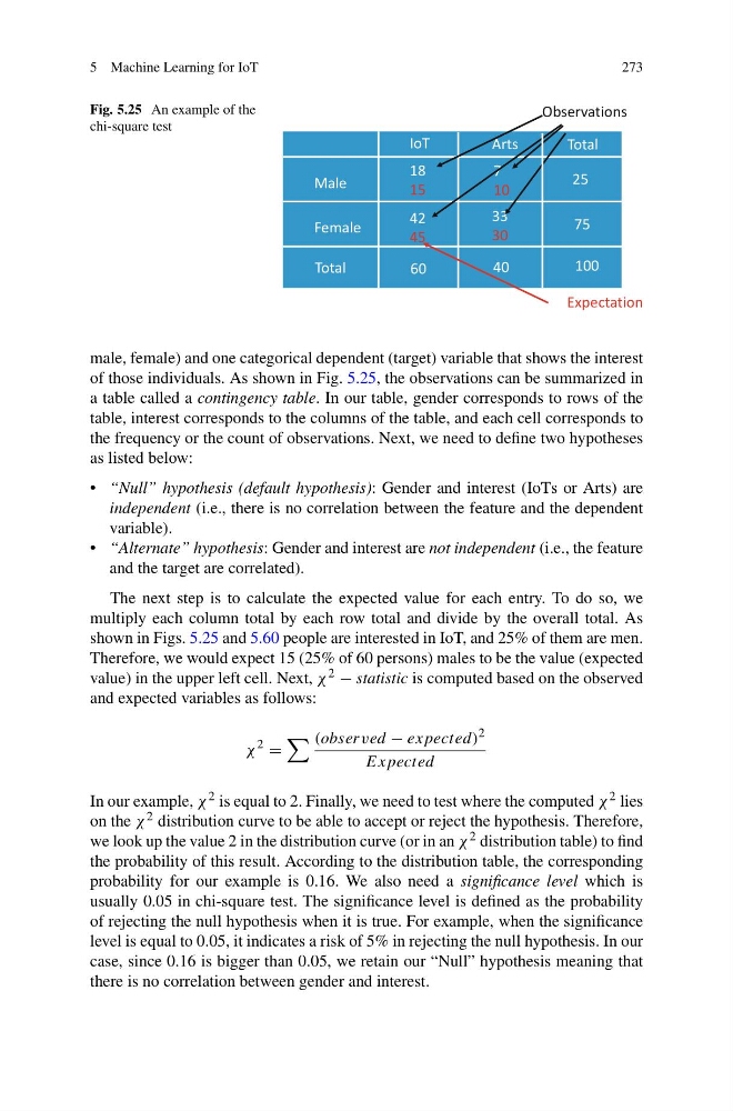
Fig. 5.25 An example of the
chi-square test
Male
Female
IoT
Arts
18
15
7
10
42
45
33
30
Observations
Total
Total
25
75
100
60
40
Expectation
male, female) and one categorical dependent (target) variable that shows the interest
of those individuals. As shown in Fig. 5.25, the observations can be summarized in
a table called a contingency table. In our table, gender corresponds to rows of the
table, interest corresponds to the columns of the table, and each cell corresponds to
the frequency or the count of observations. Next, we need to define two hypotheses
as listed below:
• “Null” hypothesis (default hypothesis): Gender and interest (IoTs or Arts) are
independent (i.e., there is no correlation between the feature and the dependent
variable).
• “Alternate” hypothesis: Gender and interest are not independent (i.e., the feature
and the target are correlated).
The next step is to calculate the expected value for each entry. To do so, we
multiply each column total by each row total and divide by the overall total. As
shown in Figs. 5.25 and 5.60 people are interested in IoT, and 25% of them are men.
Therefore, we would expect 15 (25% of 60 persons) males to be the value (expected
value) in the upper left cell. Next, χ 2 − statistic is computed based on the observed
and expected variables as follows:
χ
2
=
(observed − expected)
2
Expected
In our example, χ 2 is equal to 2. Finally, we need to test where the computed χ 2 lies
on the χ 2 distribution curve to be able to accept or reject the hypothesis. Therefore,
we look up the value 2 in the distribution curve (or in an χ 2 distribution table) to find
the probability of this result. According to the distribution table, the corresponding
probability for our example is 0.16. We also need a significance level which is
usually 0.05 in chi-square test. The significance level is defined as the probability
of rejecting the null hypothesis when it is true. For example, when the significance
level is equal to 0.05, it indicates a risk of 5% in rejecting the null hypothesis. In our
case, since 0.16 is bigger than 0.05, we retain our “Null” hypothesis meaning that
there is no correlation between gender and interest.
273
Fig. 5.25 An example of the
chi-square test
Male
Female
IoT
Arts
18
15
7
10
42
45
33
30
Observations
Total
Total
25
75
100
60
40
Expectation
male, female) and one categorical dependent (target) variable that shows the interest
of those individuals. As shown in Fig. 5.25, the observations can be summarized in
a table called a contingency table. In our table, gender corresponds to rows of the
table, interest corresponds to the columns of the table, and each cell corresponds to
the frequency or the count of observations. Next, we need to define two hypotheses
as listed below:
• “Null” hypothesis (default hypothesis): Gender and interest (IoTs or Arts) are
independent (i.e., there is no correlation between the feature and the dependent
variable).
• “Alternate” hypothesis: Gender and interest are not independent (i.e., the feature
and the target are correlated).
The next step is to calculate the expected value for each entry. To do so, we
multiply each column total by each row total and divide by the overall total. As
shown in Figs. 5.25 and 5.60 people are interested in IoT, and 25% of them are men.
Therefore, we would expect 15 (25% of 60 persons) males to be the value (expected
value) in the upper left cell. Next, χ 2 − statistic is computed based on the observed
and expected variables as follows:
χ
2
=
(observed − expected)
2
Expected
In our example, χ 2 is equal to 2. Finally, we need to test where the computed χ 2 lies
on the χ 2 distribution curve to be able to accept or reject the hypothesis. Therefore,
we look up the value 2 in the distribution curve (or in an χ 2 distribution table) to find
the probability of this result. According to the distribution table, the corresponding
probability for our example is 0.16. We also need a significance level which is
usually 0.05 in chi-square test. The significance level is defined as the probability
of rejecting the null hypothesis when it is true. For example, when the significance
level is equal to 0.05, it indicates a risk of 5% in rejecting the null hypothesis. In our
case, since 0.16 is bigger than 0.05, we retain our “Null” hypothesis meaning that
there is no correlation between gender and interest.