

5 Machine Learning for IoT
263
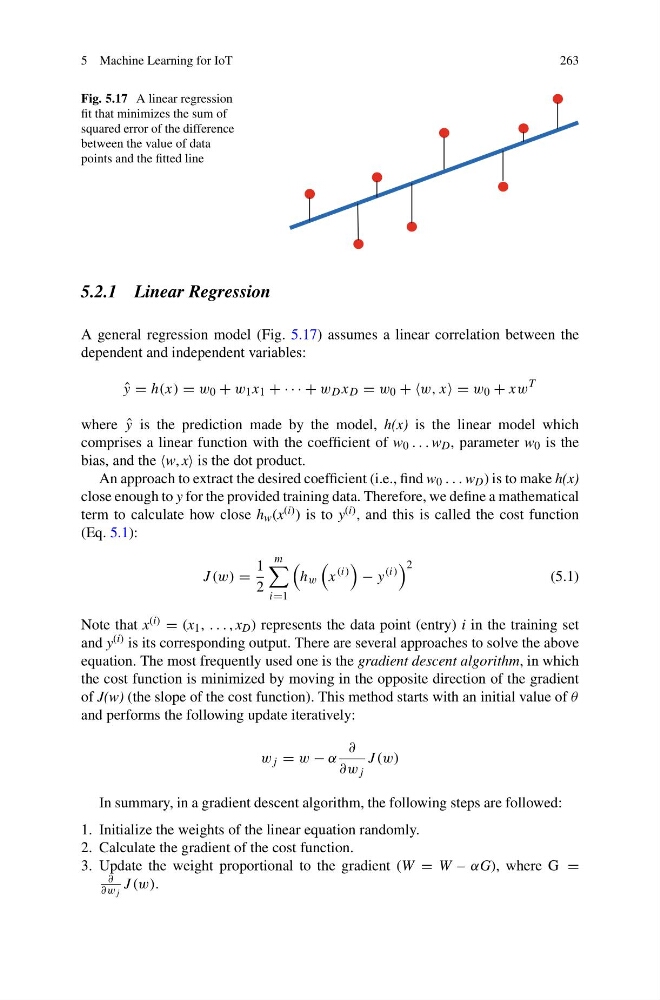
Fig. 5.17 A linear regression
fit that minimizes the sum of
squared error of the difference
between the value of data
points and the fitted line
5.2.1 Linear Regression
A general regression model (Fig. 5.17) assumes a linear correlation between the
dependent and independent variables:
ˆ
y = h(x) = w 0 + w 1 x 1 + · · · + w D x D = w 0 + w, x = w 0 + xw
T
where ˆ
y is the prediction made by the model, h(x) is the linear model which
comprises a linear function with the coefficient of w 0 . . . w D , parameter w 0 is the
bias, and the w, x is the dot product.
An approach to extract the desired coefficient (i.e., find w 0 . . . w D ) is to make h(x)
close enough to y for the provided training data. Therefore, we define a mathematical
term to calculate how close h w (x (i) ) is to y (i) , and this is called the cost function
(Eq. 5.1):
J (w) =
1
2
m
i=1
h w
x
(i)
− y
(i)
2
(5.1)
Note that x (i) = (x 1 , . . . , x D ) represents the data point (entry) i in the training set
and y (i) is its corresponding output. There are several approaches to solve the above
equation. The most frequently used one is the gradient descent algorithm, in which
the cost function is minimized by moving in the opposite direction of the gradient
of J(w) (the slope of the cost function). This method starts with an initial value of θ
and performs the following update iteratively:
w j = w − α
∂
∂w j
J (w)
In summary, in a gradient descent algorithm, the following steps are followed:
1. Initialize the weights of the linear equation randomly.
2. Calculate the gradient of the cost function.
3. Update the weight proportional to the gradient (W = W – αG), where G =
∂
∂w j
J (w).
263
Fig. 5.17 A linear regression
fit that minimizes the sum of
squared error of the difference
between the value of data
points and the fitted line
5.2.1 Linear Regression
A general regression model (Fig. 5.17) assumes a linear correlation between the
dependent and independent variables:
ˆ
y = h(x) = w 0 + w 1 x 1 + · · · + w D x D = w 0 + w, x = w 0 + xw
T
where ˆ
y is the prediction made by the model, h(x) is the linear model which
comprises a linear function with the coefficient of w 0 . . . w D , parameter w 0 is the
bias, and the w, x is the dot product.
An approach to extract the desired coefficient (i.e., find w 0 . . . w D ) is to make h(x)
close enough to y for the provided training data. Therefore, we define a mathematical
term to calculate how close h w (x (i) ) is to y (i) , and this is called the cost function
(Eq. 5.1):
J (w) =
1
2
m
i=1
h w
x
(i)
− y
(i)
2
(5.1)
Note that x (i) = (x 1 , . . . , x D ) represents the data point (entry) i in the training set
and y (i) is its corresponding output. There are several approaches to solve the above
equation. The most frequently used one is the gradient descent algorithm, in which
the cost function is minimized by moving in the opposite direction of the gradient
of J(w) (the slope of the cost function). This method starts with an initial value of θ
and performs the following update iteratively:
w j = w − α
∂
∂w j
J (w)
In summary, in a gradient descent algorithm, the following steps are followed:
1. Initialize the weights of the linear equation randomly.
2. Calculate the gradient of the cost function.
3. Update the weight proportional to the gradient (W = W – αG), where G =
∂
∂w j
J (w).