

5.4 Results of Case Studies
73
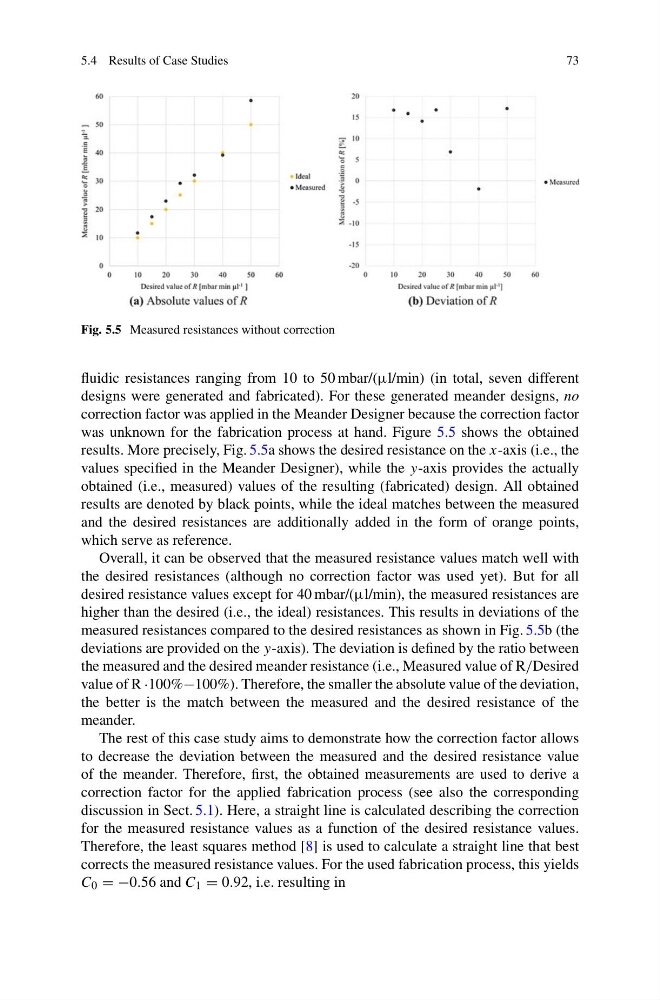
Fig. 5.5 Measured resistances without correction
fluidic resistances ranging from 10 to 50 mbar/(μl/min) (in total, seven different
designs were generated and fabricated). For these generated meander designs, no
correction factor was applied in the Meander Designer because the correction factor
was unknown for the fabrication process at hand. Figure 5.5 shows the obtained
results. More precisely, Fig. 5.5a shows the desired resistance on the x-axis (i.e., the
values specified in the Meander Designer), while the y-axis provides the actually
obtained (i.e., measured) values of the resulting (fabricated) design. All obtained
results are denoted by black points, while the ideal matches between the measured
and the desired resistances are additionally added in the form of orange points,
which serve as reference.
Overall, it can be observed that the measured resistance values match well with
the desired resistances (although no correction factor was used yet). But for all
desired resistance values except for 40 mbar/(μl/min), the measured resistances are
higher than the desired (i.e., the ideal) resistances. This results in deviations of the
measured resistances compared to the desired resistances as shown in Fig. 5.5b (the
deviations are provided on the y-axis). The deviation is defined by the ratio between
the measured and the desired meander resistance (i.e., Measured value of R/Desired
value of R ·100%−100%). Therefore, the smaller the absolute value of the deviation,
the better is the match between the measured and the desired resistance of the
meander.
The rest of this case study aims to demonstrate how the correction factor allows
to decrease the deviation between the measured and the desired resistance value
of the meander. Therefore, first, the obtained measurements are used to derive a
correction factor for the applied fabrication process (see also the corresponding
discussion in Sect. 5.1). Here, a straight line is calculated describing the correction
for the measured resistance values as a function of the desired resistance values.
Therefore, the least squares method [8] is used to calculate a straight line that best
corrects the measured resistance values. For the used fabrication process, this yields
C 0 = −0.56 and C 1 = 0.92, i.e. resulting in
73
Fig. 5.5 Measured resistances without correction
fluidic resistances ranging from 10 to 50 mbar/(μl/min) (in total, seven different
designs were generated and fabricated). For these generated meander designs, no
correction factor was applied in the Meander Designer because the correction factor
was unknown for the fabrication process at hand. Figure 5.5 shows the obtained
results. More precisely, Fig. 5.5a shows the desired resistance on the x-axis (i.e., the
values specified in the Meander Designer), while the y-axis provides the actually
obtained (i.e., measured) values of the resulting (fabricated) design. All obtained
results are denoted by black points, while the ideal matches between the measured
and the desired resistances are additionally added in the form of orange points,
which serve as reference.
Overall, it can be observed that the measured resistance values match well with
the desired resistances (although no correction factor was used yet). But for all
desired resistance values except for 40 mbar/(μl/min), the measured resistances are
higher than the desired (i.e., the ideal) resistances. This results in deviations of the
measured resistances compared to the desired resistances as shown in Fig. 5.5b (the
deviations are provided on the y-axis). The deviation is defined by the ratio between
the measured and the desired meander resistance (i.e., Measured value of R/Desired
value of R ·100%−100%). Therefore, the smaller the absolute value of the deviation,
the better is the match between the measured and the desired resistance of the
meander.
The rest of this case study aims to demonstrate how the correction factor allows
to decrease the deviation between the measured and the desired resistance value
of the meander. Therefore, first, the obtained measurements are used to derive a
correction factor for the applied fabrication process (see also the corresponding
discussion in Sect. 5.1). Here, a straight line is calculated describing the correction
for the measured resistance values as a function of the desired resistance values.
Therefore, the least squares method [8] is used to calculate a straight line that best
corrects the measured resistance values. For the used fabrication process, this yields
C 0 = −0.56 and C 1 = 0.92, i.e. resulting in